A Lightweight Real-time Stereo Depth Estimation Network with

Dynamic Upsampling Modules

Yong Deng

1 a

, Jimin Xiao

2 b

and Steven Zhiying Zhou

1,3

Department of Electrical and Computer Engineering, National University of Singapore, 117583, Singapore

Department of Electrical and Electronic Engineering, Xi’an Jiaotong-Liverpool University, Suzhou,

Jiangsu, 215123, P.R.China

National University of Singapore Suzhou Research Institute, Suzhou, Jiangsu, 215123, P.R.China

Keywords:

Stereo Matching, Depth Estimation, Deep Learning, Dynamic Upsampling.

Abstract:

Deep learning based stereo matching networks achieve great success in the depth estimation from stereo image

pairs. However, current state-of-the-art methods usually are computationally intensive, which prevents them

from being applied in real-time scenarios or on mobile platforms with limited computational resources. In

order to tackle this shortcoming, we propose a lightweight real-time stereo matching network for disparity

estimation. Our network adopts the efﬁcient hierarchical Coarse-To-Fine (CTF) matching scheme, which starts

matching from the low-resolution feature maps, and then upsamples and reﬁnes the previous disparity stage by

stage until the full resolution. We can take the result of any stage as output to trade off accuracy and runtime.

We propose an efﬁcient hourglass-shaped feature extractor based on the latest MobileNet V3 to extract multi-

resolution feature maps from stereo image pairs. We also propose to replace the traditional upsampling method

in the CTF matching scheme with the learning-based dynamic upsampling modules to avoid blurring effects

caused by conventional upsampling methods. Our model can process 1242 × 375 resolution images with 35-

68 FPS on a GeForce GTX 1660 GPU, and outperforms all competitive baselines with comparable runtime on

the KITTI 2012/2015 datasets.

1 INTRODUCTION

Depth estimation is a fundamental problem in com-

puter vision, with numerous applications including

3D reconstruction (Izadi et al., 2011; Alexiadis et al.,

2012), robotics (Schmid et al., 2013; Mancini et al.,

2016; Ye et al., 2017; Wang et al., 2017), augmented

reality (Alhaija et al., 2018; Zenati and Zerhouni,

2007), etc. Stereo matching is a passive depth esti-

mation method based on stereo triangulation between

two rectiﬁed images taken from different viewpoints

with a slight displacement. By stereo matching, we

can obtain the disparity between corresponding pixels

in the stereo images pair, which can be further trans-

formed into depth information according to the focal

length and the stereo camera’s baseline.

Unlike active depth sensors (e.g., time-of-ﬂight

cameras, structured light cameras, and LiDAR),

stereo matching only relies on dual cameras with-

out the need for a particular illumination component,

https://orcid.org/0000-0003-0987-2182

https://orcid.org/0000-0002-9416-2486

making it signiﬁcantly more affordable and energy-

efﬁcient. Therefore, stereo depth estimation is espe-

cially suitable for mobile platforms with strict power

restrictions.

Stereo matching has been studied for decades (Lu-

cas et al., 1981; Hamzah and Ibrahim, 2016), where

the algorithms can be classiﬁed into local or global

approaches in general. Recently, deep convolutional

neural networks (CNN) have been adopted in this

feild (Mayer et al., 2016; Kendall et al., 2017) and

achieve signiﬁcant progress. Deep neural networks

can learn to incorporate the context information and

thus better handle the ill-posed regions such as occlu-

sion areas, repeated patterns, and textureless regions.

Despite the remarkable advances, deep neural

networks tend to consume large amounts of com-

putational power, leading to signiﬁcant process-

ing time. Most approaches on the KITTI stereo

2012/2015 leaderboards (Geiger et al., 2012; Menze

and Geiger, 2015) cannot achieve real-time process-

ing even though with a high-end GPU. For example,

CSPN (Cheng et al., 2019), the current state-of-the-

Deng, Y., Xiao, J. and Zhou, S.

A Lightweight Real-time Stereo Depth Estimation Network with Dynamic Upsampling Modules.

DOI: 10.5220/0010197607010710

In Proceedings of the 16th International Joint Conference on Computer Vision, Imaging and Computer Graphics Theory and Applications (VISIGRAPP 2021) - Volume 5: VISAPP, pages

701-710

ISBN: 978-989-758-488-6

701

art stereo matching algorithm, obtains a frame rate of

1FPS on a Titian X GPU, which is too slow for real-

time applications like augmented reality.

In this paper, we propose a lightweight real-time

stereo matching network for depth estimation. Our

network adopts the efﬁcient hierarchical Coarse-To-

Fine (CTF) matching scheme (Quam, 1987; Yin et al.,

2019), which starts matching from the low-resolution

feature maps, and then upsamples and reﬁnes the pre-

vious results stage by stage until the full resolution.

The nature of such hierarchical processing allows us

trade-off accuracy and runtime on demand, i.e., we

can take the result of any stage as output and cancel

the following processing. This is called anytime com-

putational approach in (Wang et al., 2019b).

The hierarchical CTF matching scheme is efﬁ-

cient, which results from two reasons. For one thing,

it performs correspondence search hierarchically —

it ﬁrst searches for a rough disparity value in the low-

resolution stage, and then reﬁne it by searching for

a residual disparity within a small neighborhood of

previous value in the higher resolution stage. This

strategy avoids the time-consuming full range search-

ing. For another, it upsamples the low-resolution re-

sult for the initialization in the higher resolution stage,

i.e., it propagates the result of a pixel to its neigh-

borhoods. Compared to performing a hierarchical

search in full resolution, this strategy further reduces

the computational overhead. However, this strategy

leads to a drawback — it introduces errors to the dis-

parity boundary in the upsampling process. This is

because the high-frequency information is lost in the

low-resolution disparity and cannot be recovered by

naive upsampling.

To overcome this drawback, we propose to replace

the naive upsampling method with the dynamic up-

sampling modules. The proposed module ﬁrst gener-

ates dynamic upsampling kernels for each pixel in the

high-resolution disparity. The dynamic upsampling

kernels are inferred from the high-resolution feature

map. They are both sample and spatial variant, un-

like conventional upsampling kernels. In this way, the

high-frequency information can be encoded in the dy-

namic upsampling kernels and recovered in the high-

resolution disparity by the dynamic upsampling pro-

cess effectively.

For the multi-resolution feature maps extraction,

we propose an efﬁcient hourglass-shaped feature ex-

tractor MobileNetV3-Up based on the latest Mo-

bileNetV3. Compared to original MobileNetV3, our

feature extractor aggregates the multi-scale features,

allowing the network to exploit multi-scale context in-

formation, which is essential for the stereo matching

process.

The proposed network performs stereo matching

and dynamic upsampling alternately, where the re-

sults of any stage can be taken as output (Figure 1). It

can process 1242×375 resolution image with a frame

rate range from 35 to 68 FPS on a mid-end GeForce

GTX 1660 GPU, depending on which output is ﬁ-

nally adopted. We refer our network as LiteStereo

since it is designed to be lightweight. We evalu-

ate LiteStereo on multiple stereo benchmark datasets.

The results show that it outperforms all competitive

baselines with comparable runtime.

2 RELATED WORKS

Stereo Matching. Stereo matching, or depth from

stereo, is a long-standing computer vision task that

has been studied for decades (Barnard and Fischler,

1982). Detailed surveys can be found in (Scharstein

and Szeliski, 2002; Hamzah and Ibrahim, 2016). A

stereo matching pipeline typically consists of four

steps: (1) matching costs volume computation, (2)

cost volume aggregation, (3) disparity estimation,

and (4) optional disparity reﬁnement (Scharstein and

Szeliski, 2002; Hamzah and Ibrahim, 2016). Re-

cently deep convolutional neural networks have been

adopted for stereo matching and achieve great suc-

cess, where most successful network designs also fol-

low the classical pipeline (Kendall et al., 2017; Chang

and Chen, 2018; Khamis et al., 2018; Yin et al.,

2019). Hierarchical Coarse-To-Fine (CTF) match-

ing is an essential strategy in stereo matching (Quam,

1987), since it reduces both computational complex-

ity and matching ambiguity. HD3 (Yin et al., 2019)

proposes a stereo network following this strategy and

achieve state-of-the-art performance. MADNet (To-

nioni et al., 2019) proposes a real-time self-adaptive

network which can perform online adaptation in real-

time. Our work also adopts the hierarchical CTF

matching strategy to achieve real-time processing.

Efﬁcient Backbone Networks. Like the networks

for many other tasks, such as image classiﬁcation (He

et al., 2016), object detection (Lin et al., 2017) and

pose estimation (Sun et al., 2019), stereo match-

ing networks also need a backbone network for fea-

ture extraction. Efﬁcient backbone networks have

been an active research area in recent years. Mo-

bileNet (Howard et al., 2017) improves computa-

tion efﬁciency substantially by introducing depth-

wise separable convolution. The following work Mo-

bileNet V2 (Sandler et al., 2018) employs a resource-

efﬁcient block with inverted residuals and linear bot-

tlenecks. MobileNet V3 (Howard et al., 2019) uses

a combination of these layers as building blocks

VISAPP 2021 - 16th International Conference on Computer Vision Theory and Applications

702

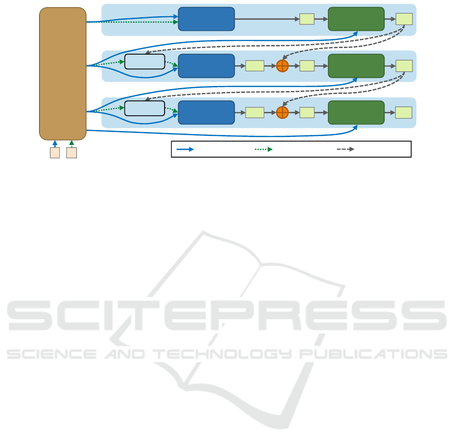
Stereo

Matching

MobileNet

V3-Up

Feature

Extractor

Stereo

Matching

Stereo

Matching

Warping

𝐷

𝑠𝑡

𝐷

𝑟𝑒𝑠

𝐷

𝑟𝑒𝑠

Dynamic

Upsampling

Dynamic

Upsampling

Dynamic

Upsampling

𝐷

𝑢𝑝

𝐷

𝑢𝑝

𝐷

𝑢𝑝

𝐷

𝑠𝑡

𝐷

𝑠𝑡

1/2

𝐼

𝐿

𝐼

𝑅

Input: Stereo Image Pair

Left feature flow Right feature flow Upsampled disp.

Stage 1

Stage 2

Stage 3

Figure 1: Network architecture of LiteStereo, which consists of a pyramid feature extractor and three stages for stereo match-

ing and dynamic upsampling. D

denotes the disparity map with the scale of 1/2

. The dynamic upsampling ratio is 2 for

Stage 1 & 2, and 4 for Stage 3. See text for details.

and exploits network architecture search algorithms

for network design. Apart from MobileNet fam-

ily, there are other efﬁcient backbone networks like

SqueezeNet (Iandola et al., 2016), ShufﬂeNet (Zhang

et al., 2018), ShiftNet (Wu et al., 2018), etc.

Depth Image Upsampling. As pointed out above, we

need a more elaborate upsampling method to recover

the high-frequency information in the upsampled dis-

parity so as to avoid the edge blurring effect. There

are many works on depth image upsampling (Eich-

hardt et al., 2017). Joint upsampling approaches (Li

et al., 2016; Hui et al., 2016) use feature maps as

guidance by merely concatenating the feature maps

of the color image and the depth image. PAC (Su

et al., 2019) predicts spatially varying kernels from

the guidance and applies them to the feature maps of

depth image for upsampling. Our dynamic upsam-

pling module is more concise and closely integrated

with the hierarchical CTF framework.

3 METHODOLOGY

The architecture overview of the proposed LiteStereo

is shown in Figure 1. The network takes a stereo

image pair I

as input, and output six disparity

maps D

with different accu-

racy successively, where the superscript of D

denotes

that the resolution is 1/2

of the full one, and st, up

denote that the disparity is produced by stereo match-

ing module and dynamic upsampling module respec-

tively.

For each input image, the MobileNetV3-Up fea-

ture extractor computes a feature pyramid that con-

sists of feature maps of different scales (1/16, 1/8,

1/4, 1). For a better trade-off between accuracy and

runtime, all computation is performed on demand.

For example, when we start with the stereo matching

module in Stage 1, only the features with the scale

of 1/2

are computed. This stereo matching module

produces a coarse disparity map D

as the ﬁrst output

of the network. If time is permitted, we continue with

the dynamic upsampling module in Stage 1. At this

time, the feature computation in MobileNetV3-Up re-

sumes from where it has stopped and outputs the left

image feature with a scale of 1/2

. The dynamic up-

sampling module increases the resolution of D

and

produces an upsampled disparity map D

with higher

resolution and accuracy.

Stage 2 follows a similar process as Stage 1, ex-

cept that it uses the disparity D

from the previous

stage as initialization, which is achieved by the warp-

ing operation. The output of the stereo matching mod-

ule in Stage 2 is a residual disparity D

res

, which is

added to the initial disparity D

to obtain the whole

disparity D

. Stage 3 follows the same process, in

which the stereo disparity map D

is upsampled to

full resolution D

via the dynamic upsampling mod-

ule with an upsampling ratio of 4.

In the rest of this section, we will introduce the de-

tails of the feature extractor, stereo matching module,

and dynamic upsampling module.

3.1 Feature Extractor

In order to keep the network lightweight and efﬁcient,

we adopt the latest MobileNetV3 (Howard et al.,

2019) as backbone for feature extraction. However,

the original MobileNetV3 is not suitable for the stereo

matching task. Since stereo matching is a pixel-to-

pixel task, high spatial resolution feature maps are

required for matching cost evaluation. However, the

A Lightweight Real-time Stereo Depth Estimation Network with Dynamic Upsampling Modules

703

high-resolution features in MobileNetV3 are in shal-

low layers, which means their receptive ﬁelds are

small and lack semantic information. Therefore, in-

spired by the U-Net (Ronneberger et al., 2015), we

add an expansion part to MobileNetV3 to aggregate

the low-scale feature with the high-scale one, so as

to exploit the context information from a larger re-

ceptive ﬁeld and obtain more semantic meaning. We

use a single 3 × 3 2D convolution layer for feature

aggregation. Thus, the increased computation over-

head is slight. The detailed network architecture can

be found in Table 1, where Operator 1-6 are the same

as in MobileNetV3-Small (Howard et al., 2019).

3.2 Stereo Matching Module

The architecture of the stereo matching module is il-

lustrated in Figure 2. The stereo matching module

takes as input the left and (warped) right feature maps

in order to compute a disparity map. Note that the

right feature maps for Stage 2 & 3 are warped accord-

ing to the disparity of previous stage:

R,wp

(x,y) = F

(x + D

init

(x,y),y), (1)

where F

R,wp

denotes the wraped feature map, F

de-

notes the right feature map, D

init

denotes the disparity

map for initialization, x,y denote the horizontal and

vertical coordinates on the 2D image plane, the super-

script l denotes the scale 1/2

. The right feature map

for Stage 1 does not need to be warped since no previ-

ous disparity is available. This is equivalent to warp-

ing with an all-zero disparity map, i.e., F

R,wp

= F

The stereo matching consists of three steps:

1) Cost Volume Computation. Given the left F

and warped right feature maps F

R,wp

, the module ﬁrst

computes a preliminary cost volume C

pre

(c,d,x, y) = F

(c,x,y) − F

R,wp

(c,x + d,y), (2)

where c denotes the index of feature channels, d de-

notes the disparity, x, y denote the horizontal and ver-

tical coordinates on the 2D image plane.

The resulting cost volume is a 4D volume with

size C × D × H × W , where C denotes the number

of feature channels of the feature map, D denotes the

number of disparities under consideration, H ×W is

the size of feature maps. The C

pre

(:,d,x, y) entry is

a distance vector that describes the matching cost be-

tween the two pixels F

(x,y) and F

R,wp

(x + d,y).

The search range (the disparities under considera-

tion) ranges from 0 to 11 for Stage 1, and from -2 to 2

for Stage 2 & 3. Note that the search range in a low-

scale feature map is equivalent to 2

times of it in the

full resolution feature map. For example, the search

𝐹

𝐿

𝐹

𝑅,𝑤𝑝

Left/right

Feature Maps

Cost Volume

Computaiton

Conv

Cost Volume

Aggregation

Soft

argmin

Disparity

Estimation

𝐷

Output

Disparity

Figure 2: Stereo matching module that performs stereo

matching between the left feature map and the (warped)

right feature map. See text for details.

range ±2 for Stage 2 / 3 is equivalent to ±16/ ± 8

pixel in the full resolution.

2) Cost Volume Aggregation. The preliminary cost

volume usually is noisy due to the matching ambigu-

ity, occlusion, or blurring in the input images. To re-

duce the noise, a cost volume aggregation step is often

applied (Hamzah and Ibrahim, 2016). We implement

the cost volume aggregation with 3D convolutional

layers (Chang and Chen, 2018). We expect the 3D

CNN learns to locally aggregate the cost by exploit-

ing the context information, and produces a 3D cost

volume with the size of D ×H ×W . The details of 3D

CNN can be found in Table 1.

3) Disparity Estimation. Given the estimated 3D

cost volume C

, a naive way to estimate the dispar-

ity map would be the winner-take-all (WTA) strategy,

where the disparity with the lowest cost would be cho-

sen as the output:

D(x,y) = argmin

(d,x,y). (3)

However, the WTA strategy cannot provide disparity

with sub-pixel accuracy. Moreover, it blocks most of

the backward propagation path during network train-

ing due to the non-differentiable argmin operation.

Therefore, we adopt the soft argmin for disparity es-

timation as suggested by (Kendall et al., 2017):

res

(x,y) =

∑

d ·

exp(−C

(d,x,y))

∑

exp(−C

,x,y))

. (4)

The estimated disparity residual D

res

is added to the

initial disparity D

init

to obtain whole disparity D

Again, since there is no initial disparity for Stage 1,

we have D

res

= D

at Stage 1.

3.3 Dynamic Upsampling Module

The proposed dynamic upsampling module is in-

spired by (Jia et al., 2016; Wang et al., 2019a). The

dynamic upsampling process is demonstrated in Fig-

ure 3. Each pixel in upsampled disparity is calcu-

lated as the weighted sum of the supported window

in low-resolution disparity centered at the reference

pixel, where the weights are deﬁned by the predicted

VISAPP 2021 - 16th International Conference on Computer Vision Theory and Applications

704

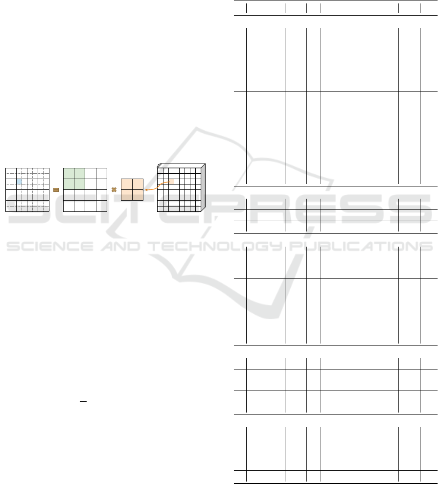
dynamic kernel. In order to achieve minimal compu-

tational overhead, we use a 2 × 2 kernel size for dy-

namic upsampling, which is similar to bilinear inter-

polation, except that the kernel weights are generated

by 2D convolutional layers. The key insight of our

dynamic upsampling module is that we predict dy-

namic upsampling kernels from the high-resolution

feature map. The predicted kernels are both sample

and spatial variant, preserving the high-frequency in-

formation. With the predicted kernels, the ﬁner de-

tails of the disparity map can be recovered in the

dynamic upsampling process. More speciﬁcally, the

predicted dynamic kernel matrix is a 4-channel fea-

ture map with the same resolution of upsampled dis-

parity. The kernel weights for each pixel are normal-

ized with softmax. The module detail can be found in

Table 1. If computational overhead is permitted, the

kernel size can be easily changed to a large size. For

example, we can use a 3 × 3 kernel size, and the pre-

dicted dynamic kernel matrix should be a 9-channel

feature map. The upsamping scale factor is 2 for

Stage 1 & 2, and 4 for Stage 3.

4 channels

Upsampled

Disparity

(2H × 2W)

Low Resolution

Disparity

(H × W)

Dynamic

Kernel

(2 × 2)

Dynamic

Kernel Matrix

(4 × 2H × 2W)

Figure 3: Dynamic upsampling process with a scale factor

of 2. Each pixel in upsampled disparity is calculated as the

weighted sum of the supported window in low resolution

disparity centered at the reference pixel, where the weights

are deﬁned by the predicted dynamic kernel matrix.

3.4 Loss Function

The network outputs the results of Operator {28, 34,

30, 36, 32, 37} successively, which correspond to

}. We upsample all out-

puts to full resolution with bilinear interpolation, and

compute the loss for each output disparity map:

L (d,

d) =

∑

i=1

smooth

−

), (5)

where d denotes the ground truth disparity, and

d de-

notes the predicted disparity, N denotes the number

of labeled pixels, smooth

denotes the smooth L1

loss function (Girshick, 2015). The losses for differ-

ent outputs are weighted differently, with weights of

0.25, 0.5, 1 for Stage 1, 2, 3 respectively.

Table 1: Network architecture of LiteStereo. s

out

denote

the scale of input and output. c

out

denote the number

of channels of input and output. (·,·) denotes concatena-

tion of two inputs. ·[:k] denotes taking the ﬁrst k channels

as input. ‘2x’ and ‘4x’ before the upsampling method de-

notes the upsampling scale. ‘conv3d x4’ denotes the layer

replicating four times with independent weights. The bold

number indicates the incoming skip link from nonsequential

layers.

# Input s

Operator s

out

MobileNetV3-Up Fearute Extractor

1 Image 1 3 conv2d, 3x3, stride 2 1/2 16

2 1 1/2 16 bneck, 3x3, stride 2 1/2

3 2 1/2

16 bneck, 3x3, stride 2 1/2

4 3 1/2

24 bneck, 3x3, stride 1 1/2

5 4 1/2

24 bneck, 3x3, stride 2 1/2

6 5 1/2

40 bneck, 3x3, stride 1 1/2

7 6 1/2

40 2x bilinear upsample 1/2

8 (4,7) 1/2

64 conv2d, 3x3, stride 1 1/2

9 8 1/2

24 2x bilinear upsample 1/2

10 (2,9) 1/2

40 conv2d, 3x3, stride 1 1/2

11 10[:4] 1/2

4 2x bilinear upsample 1/2 4

12 (1[:4],11) 1/2 8 conv2d, 3x3, stride 1 1/2 4

13 12 1/2 4 2x bilinear upsample 1 4

14 Image 1 3 conv2d, 3x3, stride 1 1 4

15 (13,14) 1 8 conv2d, 3x3, stride 1 1 4

Cost Volume Computation

16 6 1/2

40 build cost vol. 1/2

17 34 & 8 1/2

24 warp, build cost vol. 1/2

18 36 & 10 1/2

16 warp, build cost vol. 1/2

Cost Volume Aggregation

19 16 1/2

40 conv3d, 3x3x3 1/2

20 19 1/2

16 conv3d x4, 3x3x3 1/2

21 20 1/2

16 conv3d, 3x3x3 1/2

22 17 1/2

24 conv3d, 3x3x3 1/2

23 22 1/2

4 conv3d x4, 3x3x3 1/2

24 23 1/2

4 conv3d, 3x3x3 1/2

25 18 1/2

16 conv3d, 3x3x3 1/2

26 25 1/2

4 conv3d x4, 3x3x3 1/2

27 26 1/2

4 conv3d, 3x3x3 1/2

Disparity Estimation

28 21 1/2

12 soft argmin 1/2

29 24 1/2

5 soft argmin 1/2

30 29 & 34 1/2

5 sum 1/2

31 27 1/2

5 soft argmin 1/2

32 31 & 36 1/2

5 sum 1/2

Dynamic Upsampling

33 8[:12] 1/2

12 conv2d, 3x3, stride 1 1/2

34 33 & 28 1/2

1 2x dynamic upsamp. 1/2

35 10[:8] 1/2

8 conv2d, 3x3, stride 1 1/2

36 35 & 30 1/2

1 2x dynamic upsamp. 1/2

37 15 & 32 1/2

1 4x dynamic upsamp. 1 1

A Lightweight Real-time Stereo Depth Estimation Network with Dynamic Upsampling Modules

705

4 EXPERIMENTS

In this section, we evaluate our method on differ-

ent datasets and compare it with existing stereo algo-

rithms on accuracy and runtime and show that we can

achieve high-quality results and high frame rate. In

addition, we conduct ablation studies to demonstrate

the effectiveness of our network designs.

4.1 Experiment Details

4.1.1 Datasets

We trained and evaluated our method on three stereo

datasets:

1) Scene Flow (Mayer et al., 2016): a large syn-

thetic dataset containing 35454 training and 4370 test-

ing stereo image pairs, where the size of the image is

960 × 540 pixels, and the provided ground truth dis-

parity maps are dense.

2) KITTI 2012 (Geiger et al., 2012): a real-world

dataset containing 194 training and 195 testing stereo

image pairs, where the size of image is 1242 × 375

pixels, and the provided ground truth disparity maps

are sparse.

3) KITTI 2015 (Menze and Geiger, 2015): a real-

world dataset containing 200 training and 200 test-

ing stereo image pairs, where the size of the image

is 1242 × 375 pixels, and the provided ground truth

disparity maps are sparse.

4.1.2 Training Details

We implement the proposed network LiteStereo with

PyTorch, where the detailed network architecture is

shown in Table 1. Our model is trained end-to-end

using Adam (Kingma and Ba, 2014) (β

= 0.9, β

0.999) with a batch size of 6. Color normalization

is applied to the entire dataset for data preprocessing.

As for training set data augmentation, we randomly

crop the image to size H = 256 and W = 512.

Since the two KITTI datasets are too small for

training, we ﬁrst train our model on the Scene Flow

dataset and then ﬁne-tune it on the two KITTI datasets

respectively before evaluating on them. Before train-

ing, the weights of the front part of the MobileNetV3-

Up feature extractor (Operator 1-6 in Table 1) are ini-

tialized from the ImageNet pretrained MobileNetV3-

Small model (Howard et al., 2019) and then frozen.

On the Scene Flow dataset, the model is trained

for 10 epochs in total with a constant learning rate of

5 × 10

−4

. The frozen weights are unfrozen after one

training epoch. For the KITTI datasets, we ﬁne-tune

the model pretrained on the SceneFlow dataset for

300 epochs with an initial learning rate of 5 × 10

−4

The learning rate is reduced to 5 × 10

−5

after the

200th epoch. The results on KITTI datasets are av-

eraged over ﬁve randomized 80/20 train/validation

splits, which follows the evaluation protocol in (Wang

et al., 2019b).

4.1.3 Baseline Comparison

We compare our method with other four real-time

stereo matching methods: StereoNet (Khamis et al.,

2018), AnyNet (Wang et al., 2019b), MADNet (To-

nioni et al., 2019), and DispNet (Mayer et al., 2016),

where the comparison focuses on both disparity ac-

curacy and inference time. We compare different

methods only on KITTI 2012 & 2015 datasets, since

some methods did not report their results on Scene-

Flow, or the evaluation protocols are different from

each other. For a fair comparison, we perform infer-

ence with each network on the same computer with a

GeForce GTX Titan X GPU to estimate the average

runtime, where the input is a stereo image pair with

the resolution of 1242 × 375. Note that the GeForce

GTX Titan X with Maxwell

architecture we used

is signiﬁcantly inferior to the NVIDIA TITAN X with

Pascal

architecture, although they have very simi-

lar names. As for the disparity accuracy, we adopt the

performance results reported in the original papers.

4.2 Experiment Results

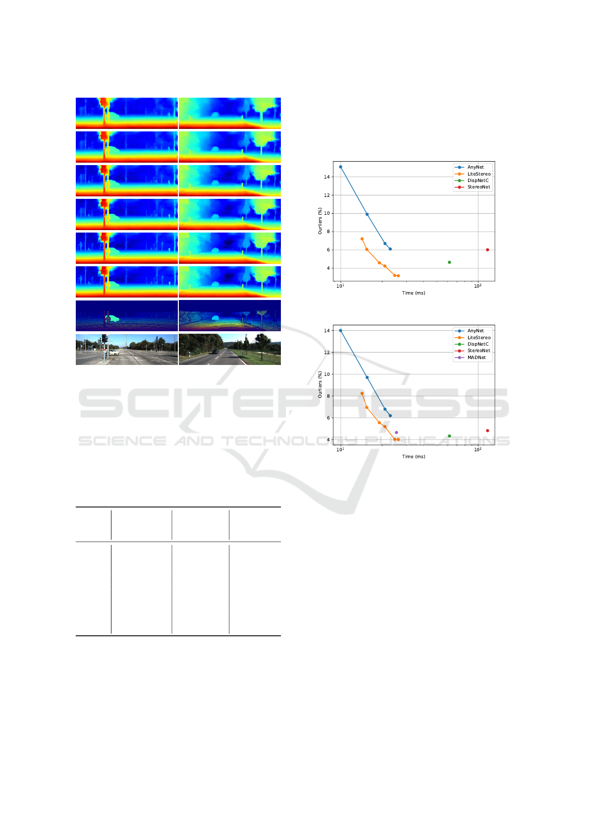
Here, we ﬁrst show the qualitative and quantitative

results of our LiteStereo on different datasets and then

compare our method with other baselines.

The qualitative results on KITTI 2015 can be

found in Figure 4. The percentage of outliers is

indicated in the ﬁgure. We only count outliers if

the disparity or ﬂow exceeds 3 pixels and 5% of its

true value, which is consistent with KITTI 2015 pa-

per (Menze and Geiger, 2015). Since the prediction is

reﬁned step by step, as more inference time is given,

more accurate results we get. Different trade-offs be-

tween accuracy and runtime can be achieved on de-

mand using one model. The quantitative results on

KITTI 2012 & 2015 and SceneFlow can be found

in Table 2. The outlier rate is used for KITTI, and

End-Point-Error (EPE) is used for SceneFlow. We

can see that the dynamic upsampling module can ef-

ﬁciently improve the accuracy with a small compu-

tational overhead. The improvement of the dynamic

upsampling module of the last stage is still signif-

icant on the SceneFlow dataset but not on KITTI

datasets. A reasonable explanation is that the ground

truth of KITTI datasets lacks valid pixels on the dis-

parity discontinuity due to its sparsity. Thus the dy-

VISAPP 2021 - 16th International Conference on Computer Vision Theory and Applications

706

Error=9.66%

Error=9.59%

Error=6.83%

Error=6.39%

Error=6.11%

Error=4.68%

Error=4.43%

Error=3.25%

Error=2.86%

Error=1.75%

Error=2.78%

Error=1.73%

GroundTruth

LeftImage

(a) (b)

Figure 4: Qualitative results on KITTI2015. The notations

of six outputs correspond to those in Figure 1. The pre-

diction is reﬁned step by step. Different trade-offs between

accuracy and runtime can be achieved on demand in one

model. Error denotes the percentage of outliers. Zoom in to

see the details.

Table 2: Runtime and outlier(%) of LiteStereo on KITTI-

2012 / KITTI-2015 datasets and EPE on SceneFlow. Lower

values are better. Runtime is measured on KITTI dataset.

“Incr.” denotes the increased time since last output, “Acc.”

denotes the accumulated time from beginning.

Time (ms) Outliers (%) EPE (px)

Output Incr. Acc. 2012 2015 SceneFlow

1. D

14.27 14.27 7.22 8.24 3.49

2. D

1.18 15.45 6.06 6.96 2.80

3. D

3.61 19.06 4.59 5.56 2.51

4. D

1.86 20.91 4.25 5.20 2.18

5. D

3.75 24.67 3.21 4.03 1.95

6. D

1.55 26.21 3.18 4.03 1.74

namic upsampling kernel CNN fails to learn reason-

able weights for the upsampling kernel prediction to

produce an accurate disparity boundary.

The comparison with other baseline is demon-

strated in Figure 5. The outlier rate is used as the met-

ric. Our method achieves a better accuracy-runtime

trade-off than all competitive real-time baselines. We

can achieve lower error rates within less runtime.

LiteStereo does not rely on any customized operator

or CUDA C/C++ programming, making it easy to be

deployed on other platforms such as mobile phones.

(a) Comparisons on KITTI 2012 dataset.

(b) Comparisons on KITTI 2015 dataset.

Figure 5: Comparisons of different baselines on KITTI

datasets. The outlier rate is used as the metric. The time

axis is logarithmic axes.

4.3 Ablation Studies

We conduct ablation studies to examine the impact of

different components of the LiteStereo network. We

evaluate different variants of our model on the Scene-

Flow dataset.

4.3.1 Feature Extractor

As described in Section 3.1, we add an expansion part

to MobileNetV3 to aggregate the multi-scale features.

In the ﬁrst ablation study, we remove the expansion

part and directly use MobileNetV3 (Operator 1-6 in

Table 1) as the feature extractor. We compare the per-

formance of MobileNetV3 and MobileNetV3-Up. To

avoid being disturbed by dynamic upsampling mod-

ule, we use a bilinear upsampler in this ablation study.

A Lightweight Real-time Stereo Depth Estimation Network with Dynamic Upsampling Modules

707

Table 3: EPE of LiteStereo with different settings evalu-

ated on SceneFlow. The number in the parentheses denotes

the reduction of EPE w.r.t. last output. “FeatExt” denotes

Feature Extractor, “feat gui” denotes feature guided joint

upsampling, “dyn up” denotes dynamic upsampling.

FeatExt MobileNetV3 MobileNetV3-Up

Upsampler bilinear bilinear feat gui dyn up

1. D

3.46 3.56 3.51 3.49

2. D

- - 3.38 2.80

3. D

2.84 (-0.62) 2.86 (-0.70) 2.84 2.51

4. D

- - 2.80 2.18

5. D

2.52 (-0.32) 2.43 (-0.43) 2.37 1.95

6. D

- - 2.41 1.74

The results is reported in Table 3. As shown in

the table, MobileNetV3 results in higher error than

MobileNetV3-Up at high-resolution output. This is

because the high-resolution features of MobileNetV3

are in shallow layers and unable to aggregate enough

context information. The resulting feature vectors for

the pixels do not contain enough information to be

distinguished from each other, which leads to am-

biguity in the stereo matching process. The feature

maps for the stereo matching module in Stage 1 are

produced in the same layer in both MobileNetV3 and

MobileNetV3-Up, which are generated by the Opera-

tor 6 in Table 1. Thus, there is no deterioration in the

ﬁrst output D

even if the MobileNetV3 is used.

4.3.2 Dynamic Upsampling Module

In order to demonstrate the effectiveness of the dy-

namic upsampling module, we compare it with tradi-

tional bilinear upsampler and a feature guided joint

upsampling method. The guided joint upsampling

module ﬁrst upsample the disparity and concatenate

it with a feature. Then, a 2D convolutional layer is

applied to it for disparity reﬁnement. We design the

guided joint upsampling module with a similar com-

putational overhead as the dynamic upsampling mod-

ule. MobileNetV3-Up is used as feature extractor.

The results are reported in Table 3. As shown in

the table, the feature guided joint upsampling only

achieves a slightly smaller error (2.37) than traditional

bilinear (2.43) at the output D

, while our dynamic

upsampling achieve signiﬁcantly lower errors than

feature guided upsampling at all outputs. We con-

clude that under such strict computational limitations,

dynamic upsampling is better than feature guided up-

sampling.

5 CONCLUSIONS

In this paper, we have proposed a lightweight efﬁ-

cient stereo matching network for disparity estima-

tion in real-time applications. Our network adopts the

efﬁcient hierarchical Coarse-To-Fine (CTF) matching

scheme. We can take the result of any stage as output

to achieve different trade-offs between accuracy and

runtime on demand in one model. We propose an efﬁ-

cient hourglass-shaped feature extractor based on the

latest MobileNetV3, which is able to aggregate more

context information from different scales. We also

propose to replace the traditional upsampling method

in the CTF matching scheme with the learning-based

dynamic upsampling modules, which improves the

accuracy signiﬁcantly with little extra overhead. In

the future, we are going to implement our network

on the mobile phone for further downstream applica-

tions.

ACKNOWLEDGEMENTS

Steven Zhiying Zhou was supported by National Key

Research and Development Program of China under

2018YFB1004904; Science and Technology Program

of Suzhou City under SYG201920. Jimin Xiao was

supported by National Natural Science Foundation of

China under 61972323; Key Program Special Fund

in XJTLU under KSF-T-02, KSF-P-02. The compu-

tational work for this article was partially performed

on resources of the National Supercomputing Centre,

Singapore (https://www.nscc.sg).

REFERENCES

Alexiadis, D. S., Zarpalas, D., and Daras, P. (2012). Real-

time, full 3-d reconstruction of moving foreground ob-

jects from multiple consumer depth cameras. IEEE

Transactions on Multimedia, 15(2):339–358.

Alhaija, H. A., Mustikovela, S. K., Mescheder, L., Geiger,

A., and Rother, C. (2018). Augmented reality meets

computer vision: Efﬁcient data generation for urban

driving scenes. International Journal of Computer Vi-

sion, 126(9):961–972.

Barnard, S. T. and Fischler, M. A. (1982). Computational

stereo. ACM Computing Surveys (CSUR), 14(4):553–

572.

Chang, J.-R. and Chen, Y.-S. (2018). Pyramid stereo match-

ing network. In Proceedings of the IEEE Conference

on Computer Vision and Pattern Recognition, pages

5410–5418.

Cheng, X., Wang, P., and Yang, R. (2019). Learning depth

with convolutional spatial propagation network. IEEE

VISAPP 2021 - 16th International Conference on Computer Vision Theory and Applications

708

transactions on pattern analysis and machine intelli-

gence.

Eichhardt, I., Chetverikov, D., and Janko, Z. (2017). Image-

guided tof depth upsampling: a survey. Machine Vi-

sion and Applications, 28(3-4):267–282.

Geiger, A., Lenz, P., and Urtasun, R. (2012). Are we ready

for autonomous driving? the kitti vision benchmark

suite. In 2012 IEEE Conference on Computer Vision

and Pattern Recognition, pages 3354–3361. IEEE.

Girshick, R. (2015). Fast r-cnn. In Proceedings of the IEEE

international conference on computer vision, pages

1440–1448.

Hamzah, R. A. and Ibrahim, H. (2016). Literature survey

on stereo vision disparity map algorithms. Journal of

Sensors, 2016.

He, K., Zhang, X., Ren, S., and Sun, J. (2016). Deep resid-

ual learning for image recognition. In Proceedings of

the IEEE conference on computer vision and pattern

recognition, pages 770–778.

Howard, A., Sandler, M., Chu, G., Chen, L.-C., Chen, B.,

Tan, M., Wang, W., Zhu, Y., Pang, R., Vasudevan, V.,

et al. (2019). Searching for mobilenetv3. In Proceed-

ings of the IEEE International Conference on Com-

puter Vision, pages 1314–1324.

Howard, A. G., Zhu, M., Chen, B., Kalenichenko, D.,

Wang, W., Weyand, T., Andreetto, M., and Adam,

H. (2017). Mobilenets: Efﬁcient convolutional neu-

ral networks for mobile vision applications. arXiv

preprint arXiv:1704.04861.

Hui, T.-W., Loy, C. C., and Tang, X. (2016). Depth map

super-resolution by deep multi-scale guidance. In Eu-

ropean conference on computer vision, pages 353–

369. Springer.

Iandola, F. N., Han, S., Moskewicz, M. W., Ashraf, K.,

Dally, W. J., and Keutzer, K. (2016). Squeezenet:

Alexnet-level accuracy with 50x fewer parame-

ters and¡ 0.5 mb model size. arXiv preprint

arXiv:1602.07360.

Izadi, S., Kim, D., Hilliges, O., Molyneaux, D., Newcombe,

R., Kohli, P., Shotton, J., Hodges, S., Freeman, D.,

Davison, A., et al. (2011). Kinectfusion: real-time 3d

reconstruction and interaction using a moving depth

camera. In Proceedings of the 24th annual ACM sym-

posium on User interface software and technology,

pages 559–568.

Jia, X., De Brabandere, B., Tuytelaars, T., and Gool, L. V.

(2016). Dynamic ﬁlter networks. In Advances in neu-

ral information processing systems, pages 667–675.

Kendall, A., Martirosyan, H., Dasgupta, S., Henry, P.,

Kennedy, R., Bachrach, A., and Bry, A. (2017). End-

to-end learning of geometry and context for deep

stereo regression. In Proceedings of the IEEE Interna-

tional Conference on Computer Vision, pages 66–75.

Khamis, S., Fanello, S., Rhemann, C., Kowdle, A.,

Valentin, J., and Izadi, S. (2018). Stereonet:

Guided hierarchical reﬁnement for real-time edge-

aware depth prediction. In Proceedings of the Euro-

pean Conference on Computer Vision (ECCV), pages

573–590.

Kingma, D. P. and Ba, J. (2014). Adam: A

method for stochastic optimization. arXiv preprint

arXiv:1412.6980.

Li, Y., Huang, J.-B., Ahuja, N., and Yang, M.-H. (2016).

Deep joint image ﬁltering. In European Conference

on Computer Vision, pages 154–169. Springer.

Lin, T.-Y., Doll

ar, P., Girshick, R., He, K., Hariharan, B.,

and Belongie, S. (2017). Feature pyramid networks

for object detection. In Proceedings of the IEEE con-

ference on computer vision and pattern recognition,

pages 2117–2125.

Lucas, B. D., Kanade, T., et al. (1981). An iterative image

registration technique with an application to stereo vi-

sion.

Mancini, M., Costante, G., Valigi, P., and Ciarfuglia, T. A.

(2016). Fast robust monocular depth estimation for

obstacle detection with fully convolutional networks.

In 2016 IEEE/RSJ International Conference on Intel-

ligent Robots and Systems (IROS), pages 4296–4303.

IEEE.

Mayer, N., Ilg, E., Hausser, P., Fischer, P., Cremers, D.,

Dosovitskiy, A., and Brox, T. (2016). A large dataset

to train convolutional networks for disparity, optical

ﬂow, and scene ﬂow estimation. In Proceedings of

the IEEE Conference on Computer Vision and Pattern

Recognition, pages 4040–4048.

Menze, M. and Geiger, A. (2015). Object scene ﬂow for au-

tonomous vehicles. In Proceedings of the IEEE Con-

ference on Computer Vision and Pattern Recognition,

pages 3061–3070.

Quam, L. H. (1987). Hierarchical warp stereo. In Readings

in computer vision, pages 80–86. Elsevier.

Ronneberger, O., Fischer, P., and Brox, T. (2015). U-net:

Convolutional networks for biomedical image seg-

mentation. In International Conference on Medical

image computing and computer-assisted intervention,

pages 234–241. Springer.

Sandler, M., Howard, A., Zhu, M., Zhmoginov, A., and

Chen, L.-C. (2018). Mobilenetv2: Inverted residu-

als and linear bottlenecks. In Proceedings of the IEEE

conference on computer vision and pattern recogni-

tion, pages 4510–4520.

Scharstein, D. and Szeliski, R. (2002). A taxonomy and

evaluation of dense two-frame stereo correspondence

algorithms. International journal of computer vision,

47(1-3):7–42.

Schmid, K., Tomic, T., Ruess, F., Hirschm

uller, H., and

Suppa, M. (2013). Stereo vision based indoor/outdoor

navigation for ﬂying robots. In 2013 IEEE/RSJ In-

ternational Conference on Intelligent Robots and Sys-

tems, pages 3955–3962. IEEE.

Su, H., Jampani, V., Sun, D., Gallo, O., Learned-Miller,

E., and Kautz, J. (2019). Pixel-adaptive convolutional

neural networks. In Proceedings of the IEEE Con-

ference on Computer Vision and Pattern Recognition,

pages 11166–11175.

Sun, K., Xiao, B., Liu, D., and Wang, J. (2019). Deep high-

resolution representation learning for human pose es-

timation. In Proceedings of the IEEE conference on

A Lightweight Real-time Stereo Depth Estimation Network with Dynamic Upsampling Modules

709

computer vision and pattern recognition, pages 5693–

5703.

Tonioni, A., Tosi, F., Poggi, M., Mattoccia, S., and Stefano,

L. D. (2019). Real-time self-adaptive deep stereo. In

Proceedings of the IEEE Conference on Computer Vi-

sion and Pattern Recognition, pages 195–204.

Wang, C., Meng, L., She, S., Mitchell, I. M., Li, T.,

Tung, F., Wan, W., Meng, M. Q.-H., and de Silva,

C. W. (2017). Autonomous mobile robot naviga-

tion in uneven and unstructured indoor environments.

In 2017 IEEE/RSJ International Conference on In-

telligent Robots and Systems (IROS), pages 109–116.

IEEE.

Wang, J., Chen, K., Xu, R., Liu, Z., Loy, C. C., and Lin, D.

(2019a). Carafe: Content-aware reassembly of fea-

tures. In Proceedings of the IEEE International Con-

ference on Computer Vision, pages 3007–3016.

Wang, Y., Lai, Z., Huang, G., Wang, B. H., Van Der Maaten,

L., Campbell, M., and Weinberger, K. Q. (2019b).

Anytime stereo image depth estimation on mobile de-

vices. In 2019 International Conference on Robotics

and Automation (ICRA), pages 5893–5900. IEEE.

Wu, B., Wan, A., Yue, X., Jin, P., Zhao, S., Golmant,

N., Gholaminejad, A., Gonzalez, J., and Keutzer, K.

(2018). Shift: A zero ﬂop, zero parameter alternative

to spatial convolutions. In Proceedings of the IEEE

Conference on Computer Vision and Pattern Recogni-

tion, pages 9127–9135.

Ye, M., Johns, E., Handa, A., Zhang, L., Pratt, P., and

Yang, G.-Z. (2017). Self-supervised siamese learning

on stereo image pairs for depth estimation in robotic

surgery. arXiv preprint arXiv:1705.08260.

Yin, Z., Darrell, T., and Yu, F. (2019). Hierarchical discrete

distribution decomposition for match density estima-

tion. In Proceedings of the IEEE Conference on Com-

puter Vision and Pattern Recognition, pages 6044–

6053.

Zenati, N. and Zerhouni, N. (2007). Dense stereo match-

ing with application to augmented reality. In 2007

IEEE International Conference on Signal Processing

and Communications, pages 1503–1506. IEEE.

Zhang, X., Zhou, X., Lin, M., and Sun, J. (2018). Shuf-

ﬂenet: An extremely efﬁcient convolutional neural

network for mobile devices. In Proceedings of the

IEEE conference on computer vision and pattern

recognition, pages 6848–6856.

VISAPP 2021 - 16th International Conference on Computer Vision Theory and Applications

710