Causal Campbell-Goodhart’s Law and Reinforcement Learning
Hal Ashton
a
Computer Science, University College London, U.K.
Keywords:
Reinforcement Learning, Goodhart’s Law, Campbell’s Law, Causal Inference, Cognitive Error.
Abstract:
Campbell-Goodhart’s law relates to the causal inference error whereby decision-making agents aim to influ-
ence variables which are correlated to their goal objective but do not reliably cause it. This is a well known
error in Economics and Political Science but not widely labelled in Artificial Intelligence research. Through a
simple example, we show how off-the-shelf deep Reinforcement Learning (RL) algorithms are not necessarily
immune to this cognitive error. The off-policy learning method is tricked, whilst the on-policy method is not.
The practical implication is that naive application of RL to complex real life problems can result in the same
types of policy errors that humans make. Great care should be taken around understanding the causal model
that underpins a solution derived from Reinforcement Learning.
1 INTRODUCTION
In many learning tasks, the learning agent has an im-
pact on a stochastic state variable through its previ-
ous actions. If when undisturbed, this variable pre-
dicts but does not reliably cause something of interest
to the agent, the agent might choose actions to tar-
get this variable thereby causing suboptimal perfor-
mance. This is related to Campbell-Goodhart’s law in
social science which is described as: ”When a mea-
sure becomes a target, it ceases to be a good measure”
(Strathern, 1997). Manheim and Garrabrant (2018)
describe it occurring ”When optimization causes a
collapse of the statistical relationship between a goal
which the optimizer intends and the proxy used for
that goal”.
In such a situation it is important to have a
causal model for the learning task so that the agent
is able to correctly separate the effect of its actions
on the world, from those which are caused by some
other mechanism. According to Pearl and Mackensie
(2018), reasoning based on correlations alone is not
sufficient to solve certain causal problems. So-called
level 2 and 3 problems on their inference ladder re-
quire concepts of causality, intervention and counter-
factual reasoning.
Recently ’Deep’ Reinforcement Learning (RL)
has had great success in the automated mastery of
learning optimal policies to hard problems such as
Chess and Go (Silver et al., 2017) and a range of
a
https://orcid.org/0000-0002-1780-9127
computer games starting with Atari (Mnih et al.,
2015) through to more advanced games like Star-
Craft (Vinyals et al., 2019) through the use of Neu-
ral networks. All of these problems have environ-
ments where there is an effect to the optimizer’s ac-
tions and yet RL has traditionally avoided discussing
causality at all
1
. Are the successes stated above made
possible because the problems have straightforward
causal dependencies? Perhaps inside the black boxes
derived during training, a causal inference technique
is found automatically. Else, are RL methods easily
confounded by simple causal problems? It seems use-
ful to know for anyone wishing to use RL for real
world applications like finance. The inability to ex-
plain AI coupled with claims as to its superhuman
abilities is termed ’enchanted determinism’ in Cam-
polo and Crawford (2020). Over-confidence and an
accountability shield are two ill-effects of this phe-
nomenon.
In this paper I present a toy-problem where an
agent is able to alter (or intervene on) a variable that
can be otherwise used to predict its reward. This prob-
lem is classified as Causal Goodhart by Mannheim
and Garrabant (Specifically metric manipulation). It
is deliberately simple and it can be solved either ana-
lytically or using a number of learning methods with-
out involving neural networks. The motivation is to
see whether problems that have an interesting causal
1
For example the canonical text in Reinforcement
Learning: Sutton and Barto (2018) makes no explicit ref-
erence to causality throughout the book.
Ashton, H.
Causal Campbell-Goodhart’s Law and Reinforcement Learning.
DOI: 10.5220/0010197300670073
In Proceedings of the 13th International Conference on Agents and Artificial Intelligence (ICAART 2021) - Volume 2, pages 67-73
ISBN: 978-989-758-484-8
Copyright
c
 2021 by SCITEPRESS – Science and Technology Publications, Lda. All rights reserved
67

structure can be solved through a naive application of
existing, off the shelf RL learning algorithms which
have had success solving complex problems.
2 THE DOG BAROMETER
PROBLEM
There is a dog living in a house in Scotland that wants
to go for a walk. The dog can observe current weather
through a window but really needs to know future
weather when it is walking.
The capricious weather of Scotland is either Rain
or Sunshine and depends on recent barometric pres-
sure only.
The barometric pressure (henceforth just pressure)
is either high or low. Future pressure depends only on
past pressure. High pressure causes sunshine more
often and low pressure causes rain more often.
The dog would like to wear its smart coat when it
is raining, but not wear it when it is sunny. Once it
has committed to its sartorial choice, the dog leaves
its house and experiences the weather during its walk.
This marks the end of the decision problem for the
dog.
Within the house there is a barometer which mea-
sures current pressure and has two states high and low.
The dog can see the barometer. The barometer also
has a button which the dog can press. The effect is to
set its reading to high.
2
2.1 Causal Structure
High pressure (P
t
= 1) causes a high barometer read-
ing (B
t
= 1) and a high chance of sunshine period
(W
t+1
= 1).
Conversely Low pressure (P
t
= 1) causes a low
barometer reading (B
t
= 1) and a higher chance of
rain next period (W
t+1
= 1).
Touching the barometer causes a high barometer
reading (B
t+1
= 1) next period regardless of the pres-
sure
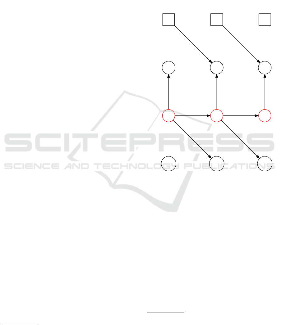
This is summarised by the DAG in Figure 1 lim-
ited to three periods. Alternatively it can be written
with the following independence statement:
P(P
t
, B
t
, W
t
|P
t−1
, B
t−1
, W
t−1
, A
t−1
) =
P(P
t
|P
t−1
).P(B
t
|P
t
, A
t−1
).P(W
t
|P
t−1
) (1)
2
The barometer use is inspired from a lecture given by
Prof Ricardo Silva at UCL
In the simplest case, Pressure has no autocorrelation:
P(P
t
|P
t−1
) = P(P
t
). This also has the effect of making
the Weather variable useless to the dog.
The effect of the dog pressing the button and set-
ting the Barometer variable B
t
is akin to that of an
atomic intervention (Pearl, 2000). This removes any
arcs from parental nodes leading to B
t
, meaning that
inference about the state of P
t
is impossible.
P
0
P
1
B
0
W
1
P
2
B
1
W
2
B
2
W
0
A
0
A
1
A
2
Figure 1: Causal diagram for dog barometer problem shown
for 3 periods. A
t
variables represent actions, B
t
pressure
readings from the barometer, P
t
the actual pressure, and W
t
the current weather. Pressure is hidden to the (canine) ob-
server. The button press makes an intervention on the state
of B
i
, accordingly all incoming arrows into B
i
should be
deleted, thereby making it useless as an indicator for P
i
.
2.2 Problem as a MDP
We will model this problem as a MDP (Markov Deci-
sion Process)
3
. Time is discretised and indexed by t.
An MDP is a tuple (S , A, R, T , S
0
, γ) where:
1. S is the set of states. The binary random weather
variable be W, with rain denoted W = 0 and sun-
shine W = 1. Pressure variable is P, with a high
state denoted P = 1 and a low state P = 0. Simi-
larly for Barometer reading B.
3
Assuming that pressure is not observable, it is better
modelled as a Partially Observable Markov Decision Pro-
cess (POMDP), but we will proceed naively ’
`
a la mode’ and
ignore the hidden variable.
ICAART 2021 - 13th International Conference on Agents and Artificial Intelligence
68

2. A is the set of actions. The dog is able to do one
of four things at any time period.
(a) Do nothing and wait a
t
= w
(b) Touch the barometer a
t
= m
(c) Put on a coat and leave their kennel a
t
= c
(d) Leave the kennel without a coat. a
t
= n
3. R : S × A :→ R is the reward function. The dog
prefers to go outside in the sun (r
nS
) with no coat,
quite likes going outside with a coat in the rain
(r
cR
) but dislikes wearing a coat in the sun (r
cS
)
and going out in the rain without a coat (r
nR
).
These four rewards are ordered r
nS
≥ r
cR
≥ r
cS
≥
r
nR
. An example assignment is shown in table 1.
Table 1: Rewards for the dog.
Rain Sun
Coat r
cR
= 4 r
cS
= −8
No Coat r
nR
= −8 r
nS
= 8
There is also an optional penalty r
wait
= −1 for
the dog when it chooses actions w and m, which
involve it waiting in the house. Whilst the dis-
count factor would seem to have a similar effect,
such a penalty is often used in practice to avoid
sparse reward signals and help the learning algo-
rithm.
4. T (s, a, s
0
) = P(s
0
|s, a) is the transition function
determining the probability of transitioning from
state s to s
0
after taking action a. It is shown in
tables 2, 3 and 4.
Table 2: P(P
t
|P
t−1
). Pressure transition: When ρ
HH
=
ρ
LL
= 0.5 there is no autocorrelation.
P(P
t
|P
t−1
) P
t−1
= Low P
t−1
= High
P
t
= Low ρ
LL
ρ
LH
= 1 − ρ
HH
P
t
= High ρ
HL
= 1 − ρ
LL
ρ
HH
Table 3: P(B
t
|P
t−1
, A
t−1
) If the button on the barometer has
been touched in the previous period (A
t−1
= 1) the proba-
bility of a high reading is 1. The α
.
coefficients correspond
to the accuracy of the barometer.
P(B
t
|P
t
, A
t−1
)
A
t−1
= 0 A
t−1
= 1
P
t
= Low P
t
= High P
t
= Low P
t
= High
B
t
= Low α
L
= 0.9 1 − α
H
0 0
B
t
= High 1 − α
L
α
H
= 0.9 1 1
Table 4: P(W
t
|P
t−1
). The ω
..
coefficients correspond to the
capriciousness of the weather.
P(W
t
|P
t−1
) P
t−1
= Low P
t−1
= High
W
t
= Rain ω
RL
= 0.9 1 − ω
SH
W
t
= Sun 1 − ω
RL
ω
SH
= 0.9
5. S
0
∈ P(S ) is a distribution over states that the
process begins at. For the initial states we draw
P
−1
= H with probability 0.5 and generate P
0
, B
0
and W
0
according to the conditional distributions
in tables 2,3 and 4 respectively.
6. γ = 0.95 is a discount factor which reflects how
much less the dog values future rewards from
present ones.
The dog must choose a policy function π : S :→ A to
maximise the following discounted sum of rewards:
arg
π
maxE

∑
t
γ
t
R(s
t
, a
t
)


π

(2)
3 METHOD
I implemented the Dog Barometer problem in Open
AI gym
4
. I then tested two Deep RL learning al-
gorithms on this problem using the StableBaselines 3
module which provides a number of implementations
of state of the art deep RL algorithms
5
. The code for
the Dog Barometer environment and tests is available
online
6
.
For each algorithm I tested the case when pres-
sure is (somehow) visible to the dog as a baseline and
when it is not. In both cases the algorithm was trained
separately 10 times.
The first learning algorithm tested was DQN,
which was shown to be successful learning how to
play Atari games in Mnih et al. (2015). It learns
through Q-learning (Sutton and Barto, 2018) and ap-
proximates the State-action function (aka Q-function)
through a neural network. The optimal policy is then
the action with the highest value for any state A mem-
ory of experiences (termed experience replay) is built
up to allow batch updates of the neural networks. This
algorithm is classified as off-policy learning, since
the algorithm estimates the value of an optimal pol-
icy without having to follow that policy during explo-
ration.
The second learning algorithm I tested was A2C
which evolved from Mnih et al. (2016). This is an
actor-critic method which estimates value and actions
functions through neural-networks. It is an on-policy
learning method, that is to say the algorithm seeks to
improve the policy it is currently following.
In both cases, I used the default parameters ac-
cording to StableBaselines 3. In particular all the neu-
ral networks were two layered, feed-forward percep-
trons of 64 neurons each with Tanh activations.
4
https://gym.openai.com/
5
https://github.com/DLR-RM/stable-baselines3
6
Environment available at https://github.com/yetiminer/
dogbarometer/
Causal Campbell-Goodhart’s Law and Reinforcement Learning
69

The A2C algorithm was trained for 20,000
episodes and the DQN algorithm, being less efficient
was trained for 100,000. These figures were chosen
for sufficient convergence properties. Default settings
from the StableBaselines3
7
module were used for
both algorithms. The resultant strategies were eval-
uated over 10,000 episodes.
4 RESULTS
In Experiment 1, pressure has no auto-correlation:
ρ
LL
= ρ
HH
= 0.5. This makes the strategy of wait-
ing for high pressure or a high barometer reading the
most efficient. We denote this strategy Π
nw
. Table
5 shows the results of the different training methods.
When Pressure is visible, the optimal strategy is re-
covered by both algos though some of the time A2C
converges on Π
nc
- wear or don’t wear coat accord-
ing to barometer. When pressure is hidden, the A2C
algorithm successfully finds the optimal strategy Π
nw
on every occasion. The DQN algorithm always con-
verges on Π
nb
; the naive strategy that involves press-
ing the barometer button if the barometer is initially
low and going outside without a coat if the barometer
is high.
Table 5: DQN trained dogs are consistently fooled into
pressing the barometer - strategy Π
nb
whilst the A2C al-
gorithm correctly recovers the optimal strategy - Π
nc
.
Exp series Pressure Hidden Mean Reward
Strategy count
Π
nc
Π
nw
Π
nb
A2C 4.80 3 7
A2C
H
TRUE 4.15 10
DQN 5.39 10
DQN
H
TRUE 2.05 10
Table 6: Strategies found when weather is auto-correlated.
Exp series Pressure Hidden Mean Reward
Strategy count
Π
nc
Π
nb
Π
nwc
Π
nbb
A2C E2 4.58 10
A2C E2 H TRUE 3.58 10
DQN E2 4.60 10
DQN E2 H TRUE 0.87 8 2
In Experiment 2 ρ
LL
= ρ
HH
= 0.75. That is to
say pressure has auto-correlation - the probability of
maintaining the same level between periods is 0.75.
This now makes waiting for high pressure less desir-
able. It also makes the weather variable useful as an
indicator independent to the barometer for the previ-
ous state of pressure. Table 6 shows the results of
the different training methods. The A2C algorithm
successfully finds the optimal strategy Π
nwc
on every
occasion. This is the strategy where the Dog exits the
house with or without a coat depending on the barom-
7
https://github.com/DLR-RM/stable-baselines3
eter unless the barometer reads low and the weather is
fine, in which case the dog will wait a period. This
balances the chance of a misreading from the barom-
eter, the penalty of going out with a coat when the
weather is sunny. The DQN algorithm mostly con-
verges on Π
nb
; the sub-optimal strategy that involves
pressing the barometer button if the barometer is ini-
tially low but also Π
nbb
which involves pressing the
barometer on every occasion except when the barom-
eter and the weather agree on a high/sun reading. This
is an improvement on Π
nb
since the weather is being
used as an indicator though is still not efficient.
5 DISCUSSION
In our experiments we saw that the DQN method
of training consistently led to the naive strategy of
pressing the barometer to ’cause’ high pressure which
would cause desirable sunny weather. In contrast
A2C avoids this pitfall and consistently finds an op-
timal strategy.
I hypothesise that this could be due to two re-
lated features of DQN; Experience replay and Off-
policy updating. Experience replay consists of the
chunking experience which is subsequently sampled
in batches to update the neural network that estimates
the state-action value (Q-value) of each state. Be-
cause prior-actions are not saved in this memory, the
distribution of rewards is not separated between those
where the button has been pressed and those where
it has not. High reward signals from not wearing a
coat after reading a legitimately high barometer read-
ing are mixed with the disappointing ones of press-
ing the barometer and exiting without a coat. Barein-
boim and Pearl (2016) call this the data-fusion prob-
lem. Secondly DQN is an off-policy learning method
- all policies are updated during learning not just the
policy that the learner is currently following. Again
this would seem to mean that the feedback from op-
timal policies where the button is not pressed is also
credited to policies where the button is pressed.
In contrast A2C does successfully navigate the
Dog-Barometer. This is a surprise given the inade-
quacy of the state signal in its ability to show when the
barometer is behaving properly. On reflection I think
this might be because this method of learning is ’on-
policy’. Learning only occurs on a policy which is
currently being used by the learner. Since the dynam-
ics of this environment are dependent on the action-
history, and in this example, the policy encodes action
history, the learner is not tripped up as easily.
In all cases I used the default 2 layer 64 neuron
feed forward MLP. It would be useful to try a recur-
ICAART 2021 - 13th International Conference on Agents and Artificial Intelligence
70

rent neural network like an LSTM Goodfellow et al.
(2016) to see how the results changed.
6 RELATED WORK
Causality within Reinforcement Learning is begin-
ning to receive mainstream attention. An introduc-
tion to the subject is given by Bareinboim (2020) and
the associated website
8
. Guo et al. (2018) provide a
more general survey of learning causality from data.
The general issues surrounding the replay-memory of
DQN erroneously mixing data generated under dif-
ferent policies are explored in Bareinboim and Pearl
(2016).
Motivated from biological/psychological perspec-
tives Gershman (2015) places causal knowledge in
model-based and model free RL and provides a novel,
simple taxonomy to identify where causal consider-
ations can come into RL. Gershman highlights re-
search that suggest model and model-free reasoning
exists within the brain and discusses how they inter-
act with reference to the Dyna architecture of Sutton
and BartoSutton (1990).
Buesing et al. (2019) present a counterfactual
learning technique in the context of POMDPS (Par-
tially observable MDPs). They show how a model
based RL approach to POMDPs can be cast in the
language of a SCM (Structural Causal Model - see
Pearl (2000)). This is important since SCMs are the
principal tool through which causal research has pro-
gressed. Counterfactual reasoning is strongly related
with off-policy learning methods since it considers
the results of actions not taken under the policy used
to generate the experience. In contrast to their use of
an SCM to generate counter-factual data to search for
better policies, for a model-free setting, they observe
that sampling from experience can in certain circum-
stances be high variance or even useless when evalu-
ating different policies. This echoes the poor perfor-
mance of DQN in our experiment.
The subject of unobserved confounding in MDPs
(termed MDPUCs) is studied in Zhang and Barein-
boim (2016). The authors point out that MDPUCs
are quite separate from POMDPS. They observe that,
to date, MDP learning algorithms do not differenti-
ate between passive data collection and data collec-
tion after actions (interventions). The authors go on
to show that standard MDP techniques as used in RL
are not guaranteed to converge to optimal policies and
present a method using counterfactual analysis to im-
prove upon existing learning algorithms.
8
https://crl.causalai.net/ Accessed August 2020.
Model based Reinforcement Learning (MBRL) is
an area of RL research typically separate from the RL
mainstream which is model-free. In it an agent builds
a representation of the world from observational data
in order to predict future observations and thereby
plan future actions and optimise a policy. Rezende
et al. (2020) study the problem of causal errors aris-
ing from partially modelled environments in RL and
show why they occur and propose a way of mitigating
them. They illustrate the problem with a simple MDP
called ’FuzzyBear’ and explicitly relate it to causal
reasoning’s concepts of interventions, backdoors and
frontdoors taken from Pearl (2000).
Goodhart’s Law in economics (Goodhart, 1984)
is analogous to Campbell’s law (Campbell, 1979) in
social science. Since both were originally communi-
cated at around the same point in time, I thought it
was important to combine the two to aid communi-
cation, as espoused in Rodamar (2018). This article
is concerned with one variant of Goodhart-Campbell
termed ’causal’ in Manheim and Garrabrant (2018).
Whilst there is a growing knowledge base on the
failure cases of AI (see for example Lehman et al.
(2020)) the relevant ones are most often examples of
what Manheim and Garrabant term ’Shared-Cause’
Campbell-Goodhart, which is an example of objective
misalignment - the AI learns to maximise the met-
ric but not the ultimate goal of the programmer. To
my knowledge, AI research has not explicitly identi-
fied Causal-Goodhart effects when discussing failure
cases. One potential example of Causal Campbell-
Goodhart is to be found in Ha and Schmidhuber
(2018), where the AI which learns an internal model
of Doom - a computer game. On occasion it would
learn strategies that would work in its model, but
would fail when used on the actual computer game.
7 CONCLUSION
Reinforcement learning has had great success learn-
ing optimal policies in a variety of game settings, of-
ten exceeding human competence in Go, Chess, Atari
games etc. It is tempting to apply this method to more
complex problems where there are hidden variables,
stochastic outcomes and non-trivial causal structures
and hope for the best. This may lead to disappoint-
ment and more seriously, bad policies being enacted.
To date, RL Research has given very little considera-
tion to causal issues, often because the causal mecha-
nisms in the canonical test cases are straightforward.
By applying RL as is to more complex problems,
there is an implicit assumption that the neural net-
works used in deep RL, are able to figure out the prob-
Causal Campbell-Goodhart’s Law and Reinforcement Learning
71

lem of understanding causality just as well as they
can learn to decode the raw vision data fed to them
in Atari Games as in Mnih et al. and turn it into win-
ning strategies. Pearl (2000) argues that certain prob-
lems cannot be solved using correlation based statis-
tics alone; to progress to the second rung of his cau-
sation ladder, interventions need to be made. RL is
a learning framework which naturally performs inter-
ventions on the environment it seeks to learn about
yet its tools do automatically account for the mathe-
matical implications of making interventions.
The dog barometer problem that I present here is
deliberately simple and the state-space given to the
learner is not ideal for a learning algorithm. RL Meth-
ods do exist for settings with hidden variables and I
have not used them here. Expanding the state space
to include previous state values and actions may solve
the problem. However I do think that the problems
in RL raised by dog barometer are not simply the re-
sult of a straw-man argument. The presence of hidden
variables in real life learning applications is almost
certain as is the existence of non-trivial causal struc-
tures whose effect may linger over arbitrarily long
timescales thereby negating the efficacy of adding
more history. Every model of a real problem will be
misspecified to some extent; it is important to under-
stand when and why this matters. The fact that the
cognitive error is sufficiently common in social sci-
ence to be named Goodhart’s Law is a good indica-
tor that this is a policy failure case which is likely
to appear again and again in real life applications of
RL. In defence of RL, the performance of the A2C
algorithm even in the face of such misspecification is
very promising and warrants further investigation to
see whether this is consistent or an artefact of the en-
vironment.
Finally, I would like to continue to build an open
library of causal problems which new RL algorithms
can be benchmarked against. Such an approach using
the OpenAI interface has already benefited RL and I
think such a library will help widen the audience of
Causal RL to general RL researchers. In parallel it
would be useful to begin to build a taxonomy of cog-
nitive errors that AI suffers from, starting by investi-
gating whether others, similar to Campbell-Goodhart
can be recreated with RL.
ACKNOWLEDGEMENTS
This work is supported by an EPSRC PhD stu-
dentship.
REFERENCES
Bareinboim, E. (2020). Towards Causal Reinforcement
Learning (CRL). In Thirty-seventh International Con-
ference on Machine Learning (ICML2020).
Bareinboim, E. and Pearl, J. (2016). Causal inference and
the data-fusion problem. Proceedings of the National
Academy of Sciences of the United States of America,
113(27):7345–7352.
Buesing, L., Weber, T., Zwols, Y., Racaniere, S., Guez, A.,
Lespiau, J.-B., and Heess, N. (2019). Woulda, Coulda,
Shoulda: Counterfactually-guided policy search. In
ICLR.
Campbell, D. T. (1979). Assessing the impact of planned
social change. Evaluation and Program Planning,
2(1):67–90.
Campolo, A. and Crawford, K. (2020). Enchanted Deter-
minism: Power without Responsibility in Artificial In-
telligence. Engaging Science, Technology, and Soci-
ety, 6:1.
Gershman, S. J. (2015). Reinforcement learning and causal
models. Oxford Handbook of Causal Reasoning,
pages 1–32.
Goodfellow, I., Bengio, Y., and Courville, A. (2016). Deep
Learning.
Goodhart, C. A. E. (1984). Problems of Monetary Man-
agement: The UK Experience. Monetary Theory and
Practice, pages 91–121.
Guo, R., Cheng, L., Li, J., Hahn, P. R., and Liu, H. (2018).
A Survey of Learning Causality with Data: Prob-
lems and Methods. ACM Computing Surveys (CSUR),
53(4):1–37.
Ha, D. and Schmidhuber, J. (2018). World Models.
Lehman, J., Clune, J., and Misevic, D. (2020). The sur-
prising creativity of digital evolution: A collection
of anecdotes from the evolutionary computation and
artificial life research communities. Artificial Life,
26(2):274–306.
Manheim, D. and Garrabrant, S. (2018). Categorizing Vari-
ants of Goodhart’s Law.
Mnih, V., Badia, A. P., Mirza, L., Graves, A., Harley,
T., Lillicrap, T. P., Silver, D., and Kavukcuoglu, K.
(2016). Asynchronous methods for deep reinforce-
ment learning. 33rd International Conference on Ma-
chine Learning, ICML 2016, 4:2850–2869.
Mnih, V., Kavukcuoglu, K., Silver, D., ..., and Hassabis, D.
(2015). Human-level control through deep reinforce-
ment learning. Nature, 518(7540):529–533.
Pearl, J. (2000). Causality: Models, reasoning and infer-
ence. Cambridge University Press.
Pearl, J. and Mackensie, D. (2018). The Book of Why: The
new science of cause and effect. Basic Books.
Rezende, D. J., Danihelka, I., Papamakarios, G., ..., and
Buesing, L. (2020). Causally Correct Partial Models
for Reinforcement Learning.
Rodamar, J. (2018). There ought to be a law! Campbell
versus Goodhart. Significance, 15(6):9.
Silver, D., Schrittwieser, J., Simonyan, K., ..., and Hassabis,
D. (2017). Mastering the game of Go without human
knowledge. Nature, 550(7676):354–359.
ICAART 2021 - 13th International Conference on Agents and Artificial Intelligence
72

Strathern, M. (1997). ‘Improving ratings’: audit in
the British University system. European Review,
5(3):305–321.
Sutton, R. S. (1990). Integrated architectures for learn-
ing, planning, and reacting based on approximat-
ing dynamic programming. In Proceedings of the
7th. International Conference on Machine Learning,
pages(1987):216–224.
Sutton, R. S. and Barto, A. G. (2018). Reinforcement Learn-
ing: An Introduction. MIT Press, 2nd edition.
Vinyals, O., Babuschkin, I., Czarnecki, W. M., ..., and
Silver, D. (2019). Grandmaster level in StarCraft
II using multi-agent reinforcement learning. Nature,
575(7782):350–354.
Zhang, J. and Bareinboim, E. (2016). Markov Decision Pro-
cesses with Unobserved Confounders: A Causal Ap-
proach.
Causal Campbell-Goodhart’s Law and Reinforcement Learning
73