
Probabilistic (k, l)-Context-Sensitive Grammar Inference with
Gibbs Sampling Applied to Chord Sequences
Henrique Barros Lopes
a
and Alan Freitas
b
Departamento de Computac¸
˜
ao, Universidade Federal de Ouro Preto, Campus Universit
´
ario Morro do Cruzeiro,
Keywords:
Grammatical Inference, Computer Music, Chord Sequence Learning, Probabilistic Context-Sensitive
Grammars, Machine Learning, Algorithmic Composition, Artificial Intelligence.
Abstract:
Grammatical inference in computer music provides us with valuable models for fields such as algorithmic
composition, style modeling, and music theory analysis. Grammars with higher accuracy can lead to models
that improve the performance of various tasks in these fields. Recent studies show that Hidden Markov Models
can outperform Markov Models in terms of accuracy, but there are no significant differences between Hidden
Markov Models and Probabilistic Context-Free Grammars (PCFGs). This paper applies a Gibbs Sampling
algorithm to infer Probabilistic (k, l)-Context-Sensitive Grammars (P(k, l)CSGs) and presents an application
of P(k, l)CSGs to model the generation of chord sequences. Our results show Gibbs Sampling and P(k, l)CSGs
can improve on PCFGs and the Metropolis-Hastings algorithm with perplexity values that are 48% lower on
average (p-value 0.0026).
1 INTRODUCTION
The inference of probabilistic grammars is a ma-
chine learning approach applied in a myriad of fields.
Works inferring grammars are used, for example, to
validate protocols (Nouri et al., 2014; Mao et al.,
2012) and to infer flow diagrams (Breuker et al.,
2016). Computational linguistics is an important
field that makes extensive use of grammatical infer-
ences (Heinz and Rogers, 2010; Jarosz, 2013; Jarosz,
2015a; Jarosz, 2015b). This field uses inferred gram-
mars to learn patterns and relationships between let-
ters in a word or words in a phrase. These patterns
depend on the expressiveness of the inferred gram-
mar. For instance, context-sensitive grammars may
define relationships between words in English spoken
language (J
¨
ager and Rogers, 2012).
While grammar defines rules that help people
write and speak clearly and correctly, music has hier-
archical theories, e.g., functional harmony, that guide
composers to write songs pleasant to listeners. This
similarity led researchers from linguistics and music
to use similar strategies to guide their work (Forsyth
and Bello, 2013).
a
https://orcid.org/0000-0002-2185-1635
b
https://orcid.org/0000-0002-1266-0204
In computer music, the grammatical inference is
useful to fields such as algorithmic composition, style
modeling, and musical theory analysis. In Section
2, we describe many applications of grammatical in-
ferences in computer music along with the gram-
matical classes inferred in each work. We observed
that Bayesian inference works better than other ap-
proaches to infer grammars, and the use of Probabilis-
tic (k, l)-Context-Sensitive Grammars (P(k, l)CSG)s
has the potential to improve the state of the art in
chord sequence modeling.
The Bayesian algorithms Gibbs Sampling (GS)
and Metropolis-Hastings (MH) (Johnson et al., 2007;
Tsushima et al., 2018a) have been used to infer Prob-
abilistic Context-Free Grammars (PCFG), which are
in the second level of Chomsky’s hierarchy. On the
other hand, P(k, l)CSGs have been applied to model
part-of-speech tags, as in (Shibata, 2014), who has
proposed an MH algorithm to infer both PCFGs and
P(k, l)CSGs. The experiments showed a P(k, l)CSG
with (k, l) = (1, 0) achieved smaller perplexity values
than the actual state of the art algorithms.
In Section 3, this paper proposes a blocked GS
algorithm to infer P(k, l)CSGs to model chord se-
quences. We show the details of the GS algorithm for
PCFGs and describe how it can be modified to infer a
P(k, l)CSG.
572
Lopes, H. and Freitas, A.
Probabilistic (k,l)-Context-Sensitive Grammar Inference with Gibbs Sampling Applied to Chord Sequences.
DOI: 10.5220/0010195905720579
In Proceedings of the 13th International Conference on Agents and Artificial Intelligence (ICAART 2021) - Volume 2, pages 572-579
ISBN: 978-989-758-484-8
Copyright
c
2021 by SCITEPRESS – Science and Technology Publications, Lda. All rights reserved

In Section 4, we describe how we conducted our
experiments by inferring PCFGs and P(k, l)CSGs to
model the Billboard data set (Burgoyne et al., 2011)
using the GS and MH algorithms. In Section 5, we
conclude our work and present suggestions for future
work.
2 GRAMMATICAL INFERENCE
2.1 Sub-regular Grammars
Markov Models (MMs) are probabilistic models de-
scribing a sequence of possible events in which each
event’s probability depends only on the state attained
in the last o events (Gagniuc, 2017). When dealing
with grammar, these events are symbols of a word,
where a word is a sequence of grammar terminal sym-
bols. Equation 1 defines a MM of order o, where X
n+1
denotes the probability of an event. These models are
equivalent to n-grams.
P(X
n+1
|X
n
, . . . , X
0
) = P(X
n+1
|X
n
, . . . , X
n−o
) (1)
Although computer music researchers often use MMs
(Bhattacharjee and Srinivasan, 2011; Nakamura et al.,
2018; Takano and Osana, 2012; Trochidis et al.,
2016), it is possible to represent the test data set with
more expressive models. The perplexity measure ρ,
defined in Equation 2, informs the joint probability of
a grammar yielding each of the word w in the test set
W .
ρ = e
(−
1
|W |
ln(
∏
w∈W
P(w|θ))
(2)
2.2 Finite Automata
A Probabilistic Finite Automaton (PFA) is a tuple
(Q,
∑
, σ, q
0
, θ) where (i) Q is a finite set of states; (ii)
∑
is the grammar alphabet; (iii) (σ : QX
∑
→ Q) is a
transition function; (iv) q
0
is its initial state; and (v) θ
is a probability vector such that |θ| is the number of
transitions in the grammar.
Extensions of Hidden Markov Models (HMM)
and PFA, such as Mondrian Hidden Markov Mod-
els (MHMMs) (Nakano et al., 2014), and variable
Markov oracles (VMO-HMM) (Wang and Dubnov,
2017), can achieve smaller perplexity values than
MMs (Tsushima et al., 2018a). These models have
been used for chord sequences (Tsushima et al.,
2018a; Wang and Dubnov, 2017), drums pattern clas-
sification (Blaß, 2013), and musical signal processing
(Nakano et al., 2014).
2.3 Context-Free Grammars
A Probabilistic Context-Free Grammar (PCFG) is a
5-tuple (N, T, R, S, θ) where (i) N is the set of non-
terminals; (ii) T is the set of terminals; (iii) R is the set
of transition rules; (iv) S ∈ N is the initial symbol; and
(v) θ is a probability vector such that |θ| is the number
of transitions. Each rule takes the form A → α, where
A ∈ N, and α = [α
1
, . . . ] : α
i
∈ N ∪ T .
PCFGs have been used for chord sequences
(Tsushima et al., 2018a), improvising follow-ups (Ki-
tani and Koike, 2010), and harmonization (Tsushima
et al., 2017). These grammars have been inferred
with Gibbs Sampling (GS), SEQUITUR (Kitani and
Koike, 2010), and the Expectation-Maximization
(EM) algorithm (Johnson et al., 2007; Tsushima et al.,
2018a; Tsushima et al., 2017; Tsushima et al., 2018b).
Bayesian approaches like GS have been shown to
achieve smaller values of perplexity than grammars
inferred with the EM algorithm (Geman and Geman,
1984).
2.4 (k, l)-Context-Sensitive Grammars
A Probabilistic Context-Sensitive Grammar (PCSG)
is a 5-tuple (N, T, R, S, θ) where (i) N is a the set of
non-terminals; (ii) T : T ∩ N = ∅ is the set of ter-
minals; (iii) R is the set of rules; (iv) S ∈ N is the
initial symbol; and (v) θ : |θ| = |R| is a probabil-
ity vector. Each rule takes the form γ → α, where
α = [α
1
, . . . ] : ∀iα
i
∈ N ∪T and γ = [γ
1
, . . . ] : ∃iγ
i
∈ N.
In other words, a PCSG considers which symbols
are surrounding a non-terminal to decide which rule
should be used.
To avoid the problem of sequences of infinite
length in PCSGs, we can use Probabilistic (k, l)-
Context-Sensitive Grammars (P(k, l)CSGs) (Shibata,
2014). A P(k, l)CSG is a PCSG where the rules fol-
low the form γ
l
Aγ
r
→ γ
l
αγ
r
such that A ∈ N, γ
l
∈
N ∪ T, γ
r
∈ N ∪ T, α ∈ N ∪ T . The variables γ
l
and
γ
r
define a rule’s right and left contexts, respectively,
and the variables k, l indicate the maximum length of
these contexts. Thus, a P(0, 0)CSG is equivalent to a
PCFG.
P(k, l)CSGs have been inferred with the
Metropolis-Hastings (MH) algorithm (Shibata,
2014). The GS algorithm could be applied to these
grammars despite its low performance. On the other
hand, GS has the potential to use all the data in the
training data set to estimate probabilities.
Probabilistic (k,l)-Context-Sensitive Grammar Inference with Gibbs Sampling Applied to Chord Sequences
573

3 INFERRING PCFGs AND PCSGs
WITH Gibbs SAMPLING
This paper proposes the use of a GS algorithm to infer
P(k, l)CSGs. The GS algorithm can use all the train-
ing data so that we might achieve lower perplexity
values for our grammar (see Equation 2). The source
code for this work is available in our repository
1
.
In Section 3.1, we briefly discuss the GS algo-
rithm. Section 3.2 discusses the general GS algo-
rithm proposed by (Johnson et al., 2007) for inferring
PCFGs. In Section 3.3, we use this algorithm as a ref-
erence for a GS algorithm for inferring P(k, l)CSGs.
3.1 Gibbs Sampling
GS (Geman and Geman, 1984) is a Monte Carlo
Markov Chain (MCMC) method that allows us to ob-
tain samples from sets with multivariate probability
distributions. Algorithm 1 describes the method. Sup-
pose we want k samples from a multivariate random
variable X. For each of these k samples (Line 1), we
generate some initial value X
i
(Line 2) and iteratively
update this value with new samples (Line 3). The ini-
tial values X
i
can be determined randomly or by some
other algorithm.
In Line 4, we determine the current probability
distribution for the vector component x
i
j
∈ X
i
. Be-
cause we have not sampled values for x
i
k
such that
k > j yet, note the conditional probability p considers
X
i
for the indices k < j and X
i−1
for k > j. In Line 5,
we sample the component x
i
j
from this distribution d.
Algorithm 1: Gibbs Sampling.
Data: k
Result: {X
1
, . . . , X
k
}
1 for i=1 to k do
2 X
i
← initial();
3 for j=1 to n = |X| do
4 d ← p(x
i
j
|x
i
1
, . . . , x
i
j−1
, x
i−1
j+1
, . . . , x
i−1
n
);
5 x
(i)
j
← sample(d);
6 end
7 end
The sample sequence X
1
, X
1
, ..., X
k
forms an ergodic
Markov Chain, where its stationary state represents
the target distribution p.
1
https://github.com/henriqueblopes/grammatical-inferences
3.2 Gibbs Sampling for PCFGs
Given the training data, the GS inference of PCFGs
(Johnson et al., 2007) defines a target distribution over
a set of syntactic trees. The GS algorithm runs until
the target distribution p is known, and θ represents the
training set appropriately.
Note that the sequence α of a PCFG can be any
combination of symbols from the set N ∪ T , making
R infinite. However, we need to estimate θ
r
, ∀r ∈ R∗
to perform the Bayesian inference of a PCFG. That is,
we need R to be finite.
Theorem 1 (Chomsky’s Normal Form Theorem).
Any context-free language can be yielded by a gram-
mar whose rules are of the form A → BC or A → a
such that A, B,C ∈ N and a ∈ T .
With Theorem 1, we ensure that if N and T are
finite, then R is finite. Thus, θ is finite. Each word a
grammar yields has at least one syntactic tree. An
applied rule sequence from the grammar’s starting
symbol until the complete word yielding defines this
tree. We can use Bayes’ rule to calculate the syntactic
tree’s t
i
probability, given a word w
i
as in Equation 3
(Johnson et al., 2007).
P(t
i
|θ, w
i
) =
P(w
i
|θ,t
i
)P(t
i
|θ)
P(w
i
|θ)
(3)
Let W be the set of all words in the training data
set. If we calculate the product in Equation 4 for
P(t
i
|θ, w
i
) and all w
i
∈ W , we will have the joint prob-
ability P(T |θ,W ) = P(t
1
,t
2
, ...t
n
|θ,W ), which is the
joint probability of all trees in the set T = {t
1
,t
2
, ...t
n
}
that yields the set W . The GS algorithm can use the
distribution P(T|θ,W ) as a target distribution.
P(T |θ,W ) =
∏
P(t
i
|w
i
, θ) (4)
As each tree probability depends on the rules’ proba-
bilities, finding the distribution P(T |θ,W ) is the same
as finding the best θ that represents W . With the target
distribution P(T |θ,W ), we need to achieve the follow-
ing goals for a PCFG with GS:
• Calculate the prior probabilities θ;
• Sample from P(T |θ,W );
• Calculate the posterior probabilities of θ.
We take the prior probabilities as a Dirichlet distri-
bution (Johnson et al., 2007) because it is conjugate
to the PCFG’s tree distribution. Which means that
if a prior distribution over trees θ is a Dirichlet dis-
tribution, then the posterior distribution is a Dirichlet
distribution (Johnson et al., 2007). This property fa-
cilitates the posteriors’ calculations.
ICAART 2021 - 13th International Conference on Agents and Artificial Intelligence
574

The inside algorithm calculates the inside table
(Johnson et al., 2007). This table represents the prob-
abilities of a given non-terminal yielding each sub-
word of w
i
. A sample of P(T |θ,W ) is then obtained
by sampling a tree t ∈ T
w
i
yielding w
i
for each i, which
can be done with Johnson’s Sample function (Johnson
et al., 2007). This function makes use of the inside ta-
ble to randomly draw a triplet ( j, B,C), where j is the
division point of w
i
, B represents a rule for sampling
t, and C represents another rule for sampling t.
With the inside table and the sample function, we
can perform the GS for our PCFG. The parameters are
the prior θ, a PCFG, the maximum number of itera-
tions, and a training data set T D. We first initialize
a tree set. Then, for each w
i
∈ W , we calculate the
inside table and sample a tree. We update the proba-
bilities by calculating the posterior distribution using
the counter of each rule used to sample trees and re-
peat these steps according to the maximum number of
iterations. At this point, the algorithm only updates
the vector θ after sampling all trees. This variation is
known as blocked Gibbs Sampling.
3.3 Gibbs Sampling for P(k, l)CSGs
Let w denote a word yielded by a PCFG rule sequence
r
1
, r
2
, ..., r
n
. Then the tree probability is the product of
all rule probabilities. In a P(k, l)CSG, we define the
context-sensitive probabilities as in Equation 5 (Shi-
bata, 2014).
P(γ
l
Aγ
r
→ γ
l
αγ
r
) = P(A → α|γ
l
, γ
r
) (5)
Equation 5 allows a PCFG to be transformed into a
P(k, l)CSG by calculating the probabilities of each
rule marginalized by the contexts γ
l
and γ
r
. This
transformation is important because it allows us to
use Theorem 1 to turn the rule set finite. Therefore,
we can generate a P(k, l)CSG with all possible rules
given by T and N.
The sampling of P(T |θ,W ) in a P(k, l)CSG is sim-
ilar to the sampling in PCFGs. The main difference is
that when we use a rule of the form γ
l
Aγ
r
→ γ
l
BCγ
r
,
we must take into account the right context of B given
by the sequence Cγ
d−1
, where γ
d−1
is the context γ
r
without its last symbol. Another difference is that we
must know whether a rule with the left or right context
is valid. For instance, at the beginning of the algo-
rithm, the starting symbol S does not have a context.
So we must forbid rules of the form γ
l
Sγ
r
→ γ
l
BCγ
r
at this step.
Algorithm 2 (Shibata, 2014; Johnson et al., 2007)
shows the steps to do the sampling. The algorithm
requires an initial word w, the left-hand side γ
l
Aγ
r
of
the initial rule, a start position I for yielding rules, an
final position K for yielding rules, the inside table IT,
a maximum left context length k and a maximum right
context length l.
Algorithm 2: Sample Tree-KL.
Data: w, γ
l
Aγ
r
, I, K, IT , k, l
Result: R
1 begin
2 if K-I=1 then
3 R ← R ∪ {γ
l
Aγ
r
→ γ
l
w
k
γ
r
};
4 else
5 cd ← categorical distribution(IT );
6 (J, B,C) ← sample(cd);
7 (γ
l
, γ
r
) ← draw context(k,l);
8 AP ← update yield();
9 (γ
l
, γ
r
) ← adjust context(AP);
10 R ← R ∪ {γ
l
Aγ
l
→ γ
l
BCγ
l
};
11 R ← sample tree KL(w, γ
l
BCγ
r−1
, I,
I + J, IT , k, l);
12 AP ← update yield();
13 (γ
l
, γ
r
) ← adjust context(AP);
14 R ← sample tree KL(w, γ
l
Cγ
r
,
I + J + 1, K, IT , k, l);
15 end
16 end
In Line 2, Algorithm 2 verifies if the starting and end-
ing positions consist of a terminal yield. If the po-
sitions represent a terminal yield, R includes the rule
γ
l
Aγ
r
→ γ
l
w
k
γ
r
, where w
k
is the terminal to be yielded
(Line 3). If the positions do not represent a terminal
yield, Line 5 calculates a categorical distribution from
IT . Line 6 samples two non-terminals (B,C) and a
position J that the recursive calls to the function will
use to calculate the new starting and ending positions.
Next, we need to decide which right and left con-
texts the yield will use. Line 7 randomly draws one
left and one right context from all possible contexts
according to its maximum lengths, k, and l. Line 8
stores the current state of the tree sampling on the
variable AP. Then, if necessary, Line 9 removes sym-
bols from γ
l
and γ
r
to guarantee their validity.
Using the non-terminals A, B,C, and the context
γ
l
, γ
r
, Line 10 includes the rule γ
l
Aγ
l
→ γ
l
BCγ
l
in the
rule list R. Line 11 calls the sampling algorithm re-
cursively, passing as left-hand side the non-terminal
B surrounded by the contexts γ
l
and Cγ
r−1
, I as yield
starting position, and I + J as the yield ending posi-
tion. Lines 12 and 13 adjust the contexts again. This
adjustment is necessary because Line 11 has changed
the current context.
Finally, Line 14 calls the sampling algorithm re-
cursively, passing as left-hand side the non-terminal
Probabilistic (k,l)-Context-Sensitive Grammar Inference with Gibbs Sampling Applied to Chord Sequences
575

C surrounded by the contexts γ
l
and Cγ
r−1
, I + J + 1
as yield starting position, and K as the yield ending
position. At the end, the rules R will contain all sam-
pled rules to yield w, representing a syntactic tree.
As the tree sampling in a P(k, l)CSG only allows
left yields, there will never be a non-terminal to the
left of w
i
. Consequently, there will never be a termi-
nal to the right of w
i
while w
i
is yielding. So, the con-
texts γ
l
and γ
r
, where w = (w
i
, w
i+1
, ..., w
j−1
, w
j
), i <
j, are sequences containing only terminals and non-
terminals respectively, that is, γ ∈ γ
r
⇒ γ ∈ T and
γ ∈ γ
r
⇒ γ ∈ N. Therefore, the probability of A ∈ N
yielding w
ik
, given γ
l
and γ
r
, can by calculated by
Equations 6 and 7.
P
γ
l
Aγ
r
,i,i
= θ
γ
l
Aγ
r
→γ
l
w
i
γ
r
(6)
P
γ
l
Aγ
r
,i,k
=
∑
γ
l
Aγ
r
→γ
l
BCγ
r
∈R
k
∑
j=i+1
θ
γ
l
Aγ
r
→γ
l
BCγ
r
P
γ
l
Bγ
d−1
,i, j
P
γ
l
Cγ
r
, j+1,k
(7)
To construct the inside table IT , we use the inside al-
gorithm modified according to Equations 6 and 7. To
infer a P(k, l)CSG with the GS, we need to run the
GS algorithm with the sampling in Algorithm 2 and
calculate IT for a P(k, l)CSG.
4 EXPERIMENTAL RESULTS
Given the algorithms described in Sections 3.2 and
3.3, we perform experiments to compare the GS and
MH algorithms to understand the influence of the val-
ues (k, l) in a P(k,l)CSG.
4.1 Data Set
The Billboard data set (Burgoyne et al., 2011) con-
tains 890 songs. Each file contains chord sequences
split into labeled musical phrases. We extracted chord
sequences from the data set Billboard to build our
data set for inferences using the same procedure as
in (Tsushima et al., 2018a): each word represents a
chord sequence, and each chord represents a gram-
mar symbol. After the extraction, we obtained a data
set of 7217 words to infer our grammar. This data set
allows us to extract the musical phrases to get words
with a length smaller than the entire song. The ad-
vantage of this approach is to obtain a data set with
a higher number of words. The source code for this
work is available in our repository
2
.
2
https://github.com/henriqueblopes/grammatical-inferences
4.2 Inference Details
The total number of unique chords was 738. We used
the same procedure as in (Tsushima et al., 2018a) to
simplify the number |N| of non-terminals N in our
grammar. We transposed all phrases to C major and
identified the 20 most frequent chords in the data set.
We then switched the other chords to a terminal node
referred to as “Other”. We split the data set into a
training data set T D with 80% of the phrases, and a
validation data set V D with the other 20%.
Table 1 summarizes the combinations of factors in
our experiment. Due to the high computational cost of
GS, we limited the factors |T D| ≤ 3000, and |N| < 6
in our experiments.
Table 1: Factors in our Experiment.
Algorithm |N| |T D| k l
MH 2 300 0 0
MH 2 300 1 0
MH 2 3000 0 0
MH 2 3000 1 0
MH 6 300 0 0
MH 6 300 1 0
GS 2 300 0 0
GS 2 300 1 0
GS 2 3000 0 0
GS 2 3000 1 0
GS 6 300 0 0
GS 6 300 1 0
We used the inference algorithms P(k, l)CSGs with
GS described in Section 3.3 and MH (Shibata, 2014)
with k = {0, 1} and l = 0. The GS with (k, l) = (0, 0)
is one of the algorithms implemented in (Tsushima
et al., 2018a). Therefore, we will compare them to
the state of the art for the Billboards data set when
performing our experiments. We run all algorithms
in a Google Cloud virtual machine N1 series, High-
CPU type, eight cores, 7.2GB of RAM, OS Debian
GNU/Linux 10. The number of iterations was 200
and we limited the number of replicates to five for
each combination of factors due to the high compu-
tational cost of GS inferences, as discussed in more
detail in Section 4.4.
4.3 Inference Validation
We used the perplexity measure to validate the in-
ferred grammar and used the cross-validation method
dividing the data set into one different data sets per
replicate. For each replicate, we calculated the aver-
age perplexity value (Equation 2) in the test set for
each run.
ICAART 2021 - 13th International Conference on Agents and Artificial Intelligence
576
4.4 Results
Figure 1 presents the box-plots for all values of per-
plexity in the y-axis for each replicate of the MH al-
gorithm. Each pair of boxplots represents executions
with (k, l) = (0, 0) and (k,l) = (0, 1).
Figure 1: Perplexity for the MH algorithm. Experiments
with a higher value of |T D| and |N| tend to achieve lower
perplexity values. Also, grammars with k = 1 led to lower
averages.
We can see that higher values of |TD| and |N| tend to
achieve lower perplexity values. Also, when N = 6,
the presence of a left context of length k = 1 led to a
smaller perplexity value.
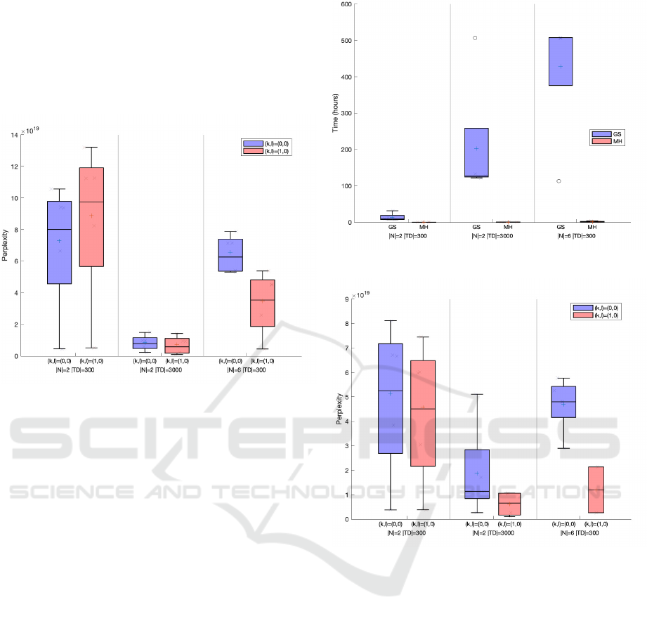
The GS samples a large number of trees at each
iteration. So GS has a much higher run time than the
MH algorithm, which is why we have a limited num-
ber of replicates. Figure 2 compares the run time of
the GS and MH.
Figure 3 shows the perplexity values obtained
with GS. In all cases, the P(k, l)CSGs have smaller
average perplexity values than PCFGs.
As in the results for the MH algorithm,
P(k, l)CSGs have smaller perplexity values than
PCFGs using GS. The perplexity becomes smaller
when we use a larger training set. This result also
indicates the presence of the left context allowed the
grammar to better represent the test sets.
In Figure 4, we compare the perplexity values
for GS and MH. The results indicate GS can achieve
lower perplexity values than MH.
We aggregated our results and used a Wilcoxon
signed paired rank-test for a paired test for the null hy-
pothesis that the average perplexity values for GS and
MH are samples from distributions with equal medi-
ans. We obtained a p-value = 0.0026 indicating that
Figure 2: GS and MH run time.
Figure 3: Perplexity Values for the GS algorithm. Gram-
mars where (k, l) = (1, 0) tend to achieve lower perplexity
values.
GS, despite its computational cost, can achieve lower
median perplexity values than MH.
5 CONCLUSIONS
We have investigated the capability of P(k, l)CSG to
represent features related to musical chord sequences
present in the Billboards data set. We used Bayesian
approaches to infer these grammars and implemented
the first blocked GS algorithm to infer P(k, l)CSGs
using the theory in (Shibata, 2014). Despite the high
computational cost GS, the presence of a left context
of size 1 provides smaller perplexity values than the
absence of contexts to represent the test sets.
These findings mean we could use the inferred
Probabilistic (k,l)-Context-Sensitive Grammar Inference with Gibbs Sampling Applied to Chord Sequences
577
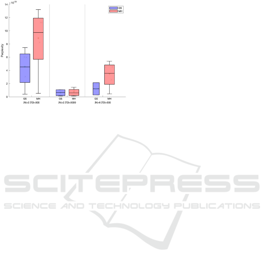
Figure 4: Perplexity Values for the GS and MH algorithms
inferring P(1, 0)CSGs.
models to perform machine learning tasks related to
chord sequences like style classification or the gener-
ation of musical phrases. The data suggest we could
improve our results by either investing in enough
computational power or developing cheaper algo-
rithms to infer grammars with k > 1 and l > 0.
ACKNOWLEDGMENTS
This work has been supported by the Brazilian Agen-
cies State of Minas Gerais Research Foundation –
FAPEMIG (APQ-00040-14); Coordination for the
Improvement of Higher Level Personnel – CAPES;
and National Council of Scientific and Technological
Development – CNPq (402956/2016-8).
REFERENCES
Bhattacharjee, A. and Srinivasan, N. (2011). Hindustani
raga representation and identification: A transition
probability based approach. International Journal of
Mind, Brain and Cognition, 2:71–99.
Blaß, M. (2013). Timbre-based drum pattern classification
using hidden markov models. In Machine Learning
and Knowledge Discovery in Databases.
Breuker, D., Matzner, M., Delfmann, P., and Becker, J.
(2016). Comprehensible predictive models for busi-
ness processes. MIS Q., 40(4):1009–1034.
Burgoyne, J., Wild, J., and Fujinaga, I. (2011). An expert
ground truth set for audio chord recognition and mu-
sic analysis. In Proceedings of the 12th International
Society for Music Information Retrieval Conference,
pages 633–638.
Forsyth, J. P. and Bello, J. (2013). Generating musical ac-
companiment using finite state transducers. In Con-
ference on Digital Audio Effects, National University
of Ireland.
Gagniuc, P. A. (2017). Markov Chains: From Theory to
Implementation and Experimentation. Wiley.
Geman, S. and Geman, D. (1984). Stochastic relaxation,
gibbs distributions, and the bayesian restoration of im-
ages. IEEE Transactions on Pattern Analysis and Ma-
chine Intelligence, PAMI-6(6):721–741.
Heinz, J. and Rogers, J. (2010). Estimating strictly piece-
wise distributions. In Proceedings of the 48th Annual
Meeting of the Association for Computational Lin-
guistics, ACL ’10, pages 886–896, Stroudsburg, PA,
USA. Association for Computational Linguistics.
Jarosz, G. (2013). Learning with hidden structure in opti-
mality theory and harmonic grammar: beyond robust
interpretive parsing. Phonology, 30(1):27–71.
Jarosz, G. (2015a). Expectation driven learning of phonol-
ogy*.
Jarosz, G. (2015b). Learning opaque and transparent inter-
actions in harmonic serialism.
J
¨
ager, G. and Rogers, J. (2012). Formal language theory:
Refining the chomsky hierarchy. Philosophical trans-
actions of the Royal Society of London. Series B, Bio-
logical sciences, 367:1956–70.
Johnson, M., Griffiths, T., and Goldwater, S. (2007).
Bayesian inference for pcfgs via markov chain monte
carlo. In Human Language Technologies 2007: The
Conference of the North American Chapter of the As-
sociation for Computational Linguistics; Proceedings
of the Main Conference, pages 139–146, Rochester,
New York. Association for Computational Linguis-
tics.
Kitani, K. and Koike, H. (2010). Improvgenerator: On-
line grammatical induction for on-the-fly improvisa-
tion accompaniment. In Proceedings of the 2010 Con-
ference on New Interfaces for Musical Expression.
Mao, H., Chen, Y., Jaeger, M., Nielsen, T., Larsen, K., and
Nielsen, B. (2012). Learning markov decision pro-
cesses for model checking. Electronic Proceedings in
Theoretical Computer Science, 103.
Nakamura, E., Nishikimi, R., Dixon, S., and Yoshii, K.
(2018). Probabilistic sequential patterns for singing
transcription. In 2018 Asia-Pacific Signal and Infor-
mation Processing Association Annual Summit and
Conference (APSIPA ASC), pages 1905–1912.
Nakano, M., Ohishi, Y., Kameoka, H., Mukai, R., and
Kashino, K. (2014). Mondrian hidden markov model
for music signal processing. In 2014 IEEE Interna-
tional Conference on Acoustics, Speech and Signal
Processing (ICASSP), pages 2405–2409.
Nouri, A., Raman, B., Bozga, M., Legay, A., and Bensalem,
S. (2014). Faster statistical model checking by means
of abstraction and learning. In Bonakdarpour, B. and
Smolka, S. A., editors, Runtime Verification, pages
340–355, Cham. Springer International Publishing.
Shibata, C. (2014). Inferring (k,l)-context-sensitive prob-
abilistic context-free grammars using hierarchical
pitman-yor processes. In Clark, A., Kanazawa, M.,
and Yoshinaka, R., editors, The 12th International
Conference on Grammatical Inference, volume 34 of
ICAART 2021 - 13th International Conference on Agents and Artificial Intelligence
578

Proceedings of Machine Learning Research, pages
153–166, Kyoto, Japan. PMLR.
Takano, M. and Osana, Y. (2012). Automatic composi-
tion system using genetic algorithm and n-gram model
considering melody blocks. In 2012 IEEE Congress
on Evolutionary Computation, pages 1–8.
Trochidis, K., Guedes, C., Anantapadmanabhan, A., and
Klaric, A. (2016). Camel: Carnatic percussion mu-
sic generation using n-gram models. In Proceedings
of the 13th Sound and Music Computing Conference.
Tsushima, H., Nakamura, E., Itoyama, K., and Yoshii, K.
(2017). Function- and rhythm-aware melody harmo-
nization based on tree-structured parsing and split-
merge sampling of chord sequences. In ISMIR.
Tsushima, H., Nakamura, E., Itoyama, K., and Yoshii,
K. (2018a). Generative statistical models with self-
emergent grammar of chord sequences. Journal of
New Music Research, 47(3):226–248.
Tsushima, H., Nakamura, E., Itoyama, K., and Yoshii,
K. (2018b). Interactive arrangement of chords and
melodies based on a tree-structured generative model.
In ISMIR.
Wang, C.-i. and Dubnov, S. (2017). Context-aware hidden
markov models of jazz music with variable markov or-
acle. In Proceedings of the Eighth International Con-
ference on Computational Creativity.
Probabilistic (k,l)-Context-Sensitive Grammar Inference with Gibbs Sampling Applied to Chord Sequences
579
