
A Raster-based Approach for Waterbodies Mesh Generation
Roberto Nisxota Menegais, Flavio Paulus Franzin, Lorenzo Schwertner Kaufmann and
Cesar Tadeu Pozzer
Curso de Ci
ˆ
encia da Computac¸
˜
ao, Universidade Federal de Santa Maria, Santa Maria, Brazil
Keywords:
Mesh Generation, Large Scale, Rasterization, GIS.
Abstract:
Meshes representing the water plane for rivers and lakes are used in a broad range of graphics applications
(e.g., games and simulations) to enhance the visual appeal of 3D virtual scenarios. These meshes can be
generated manually by an artist or automatically from supplied vector data (e.g. GIS data - Geographic Infor-
mation System), where rivers and lakes are represented by polylines and polygons, respectively. In automated
solutions, the polylines and polygons are extruded and then merged, commonly using geometric approaches,
to compose a single polygonal mesh, which is used to apply the water shaders during the rendering process.
The geometric approaches usually fail to present scalability for large datasets with a high vertex and feature
count. Also, these approaches require specific algorithms for dealing with river-river and river-lake junctions
between the entities. In opposition to geometric approaches, in this paper, we propose a raster-based solution
for efficient offline mesh generation for lakes and rivers, represented as polygons and polylines, respectively.
The solution uses a novel buffering algorithm for generating merged waterbodies from the vector data. A
modification of the Douglas-Peucker simplification algorithm is applied for reducing the vertex count and a
constrained Delaunay triangulation for obtaining the triangulated mesh. The algorithm is designed with a high
level of parallelism, which can be exploited to speed up the generation time with a multi-thread processor and
GPU computing. The results show that our solution is scalable and efficient, generating seamless polygonal
meshes for lakes and rivers in arbitrary large scenarios.
1 INTRODUCTION
Waterbody meshes are used in a broad range of appli-
cations, including games and simulations, to enhance
the visual appeal of 3D virtual scenarios. The digi-
tal portrayal of environments usually combines lakes
and rivers to represent a determined region’s hydrog-
raphy, using GIS (Geographic Information System)
vector and raster data. In this context, waterbodies re-
fer to the combination of river and lake data, being a
unique element to be rendered in a real-time graphics
application.
Even though it is an important element in vir-
tual scenarios, few studies have explored real-world
data on water mesh generation or ways to efficiently
generate it for large scenarios with a high density of
features. With the growing use of real-world loca-
tions in simulations and games (e.g. flight simula-
tors), the need for a solution to generate a polygonal
mesh based on previously generated data arises.
Usually, the river courses are represented by poly-
line datasets, and the lakes by polygons datasets,
causing a mismatch and overlap among them in the
input dataset, demanding additional data processing
to guarantee its correct mesh generation and, conse-
quently, correct rendering.
Considering this, the main aim of our solution is
to provide an offline approach to generate a polyg-
onal mesh representing the water plane of the junc-
tion between rivers and lakes represented by vector
data. The generation must guarantee a seamless junc-
tion between rivers and lakes, avoiding artifacts and
overlaps in the polygons, and be able to generate a
mesh for arbitrary large virtual scenarios.
Given a polyline dataset and a polygon dataset
representing a waterbody network, the problem can
be summarized as:
• How to efficiently generate a polygon dataset
from a polyline dataset;
• How to merge multiple datasets of rivers and lakes
into a single one;
• How to treat junctions between multiple rivers and
between lakes and rivers;
• How to achieve a minimal vertex count on the
generated polygons;
Menegais, R., Franzin, F., Kaufmann, L. and Pozzer, C.
A Raster-based Approach for Waterbodies Mesh Generation.
DOI: 10.5220/0010195501430152
In Proceedings of the 16th International Joint Conference on Computer Vision, Imaging and Computer Graphics Theory and Applications (VISIGRAPP 2021) - Volume 1: GRAPP, pages
143-152
ISBN: 978-989-758-488-6
Copyright
c
2021 by SCITEPRESS – Science and Technology Publications, Lda. All rights reserved
143

• How to efficiently triangulate the generated poly-
gons representing rivers and lakes;
• How to scale the algorithm to apply to arbitrary
large scale scenarios, considering a memory and
time constraints.
Usually, solutions to treat this problem are
geometric-based, as proposed by (Dong et al., 2003),
which treat polylines and polygons as different enti-
ties when applying the buffering algorithm, defined
by (Bhatia et al., 2013) as a zone with specified dis-
tance surrounding a spatial data feature. At the end of
the buffering process, the generated entities will over-
lap with each other. Commonly, these problems are
solved by applying a dissolve algorithm in the gen-
erated polygons; this operation consists of taking the
intersections between the edges of the buffered poly-
gons and merging them, creating vertices on the inter-
section points, as seen in Fig. 1.
InputBueringDissolve
Figure 1: Example of the buffering and dissolve operation.
The geometric approaches result in optimal ver-
tex count for the generated polygons, although they
demand individual treatments between river-river and
river-lake junctions. In this case, river-river junctions
are considered the intersection between multiple river
entities at the same vertex. This individual treatment
can also lead to high computational cost depending
on the number of entities being processed, yielding a
fast-growing algorithm on time complexity.
We propose a raster-based approach for the wa-
terbodies mesh generation, employing a rasteriza-
tion algorithm for the buffer generation. The solu-
tion eliminates the complexity of dealing with line
extrusion and junctions between line-line and line-
polygon. Also, it avoids the need to apply a dissolve
algorithm afterward. Optimizations are also proposed
to enable the application of our solution to arbitrary
large virtual scenarios.
The main contributions of our work are:
• A raster-based solution for buffering and dissolv-
ing a set of polylines and polygons data;
• An efficient approach for generating a 2D polyg-
onal mesh based on vector data;
• A scalable solution for waterbodies mesh genera-
tion that can be applied to arbitrary large scenar-
ios, with high parallelism levels.
The paper is organized as follows: Section 2 dis-
cuss related works on water mesh generation and ren-
dering. Section 3 presents an overview of the pro-
posed solution and sections 4, 5, 6, and 7 discuss each
step in-depth. Finally, in Section 8, the results are dis-
cussed and Section 9 presents the final remarks and
future work.
2 RELATED WORK
Water surface-level representation for water rendering
is commonly used when a realistic fluid simulation is
not needed, or a coarse approximation can be used.
Games and simulations apply a normal or bump map-
ping to the water surface for providing water move-
ment and the illusion of ripples and waves (Kryachko,
2005). The presence of a water plane mesh simplifies
the illumination and shading for rendering the water.
(Engel and Pozzer, 2016) proposed a framework
to generate and render river networks based on vector
data. Although the rendering results obtained were
satisfactory, the generated mesh lacked a robust junc-
tion treatment between rivers. It did not support river-
lakes junctions.
(Yu et al., 2009) proposed a scalable real-time an-
imation for rivers based on vector data, flow texture,
and a heightmap as input. The vector data used for
the application was in polygon form, meaning that
datasets representing rivers as polylines would need
a preprocessing step to convert them to polygons.
Concerning buffering algorithms, which aim is the
generation of eroded or dilated polygons, lines, and
the addition of area to points, geometric based solu-
tions were proposed (Bhatia et al., 2013), (Dong et al.,
2003). The problem with these solutions is that they
demand a dissolve algorithm after the buffering algo-
rithm to guarantee a seamless junction between fea-
tures, which adds greater complexity to the solution.
In contrast, our algorithm treats both buffering and
dissolve as a single process. Also, geometric solu-
tions may provide better results on small datasets, but
as the scale of the datasets grows, the solutions may
present a worse running time.
(Shen et al., 2018) proposes a parallel approach
for accelerated dissolved buffer generation, using In-
Memory cluster architecture. Although the solution is
highly efficient for large data and surpasses previous
solutions on buffer generation, it’s fairly complex and
uses a distributed computing approach, whereas our
approach can also deal with large data in a far simpler
manner, still using parallelization.
Regarding rasterization approaches for dealing
with vector data, (Fan et al., 2018) proposes a par-
GRAPP 2021 - 16th International Conference on Computer Graphics Theory and Applications
144

allel rasterization algorithm for vector polygon over-
lay analysis using OpenMP, they discuss in length the
benefits and errors introduced by the discretization of
the vector features, but the implementation is done us-
ing CPU cores. A GPU implementation is discussed
only in the future works. Although the goal of the
paper differs from ours, the solution is interesting to
testify the eligibility of the rasterization approach.
(Ma et al., 2018) proposed a highly efficient tech-
nique for real-time buffer analysis of large-scale spa-
tial data. Their solution uses raster-based buffering
with R-tree queries optimizations and a LOD algo-
rithm to manage rasterization quality. Although they
succeed in providing a visualization oriented paral-
lel model, their buffer generation algorithm does not
benefit from the inherited parallel nature of rasteriza-
tion. In our work, we explore buffer generation with
per-pixel parallelization using acceleration structures
proposed in (Pozzer et al., 2014) and (Engel et al.,
2016).
3 PROPOSED SOLUTION
The proposed solution performs over shapefiles rep-
resenting polylines and polygons. The shapefiles are
primarily loaded and set up in the auxiliary data struc-
tures on the GPU memory (V-RAM), ensuring par-
allelizable optimized spatial queries of the data. In
this process, a spatial hash (Pozzer et al., 2014) is
used to structure the polylines and a quadtree (Engel
et al., 2016) for the polygons. Also, to reduce pro-
cessing and memory cost, the scenario is segmented
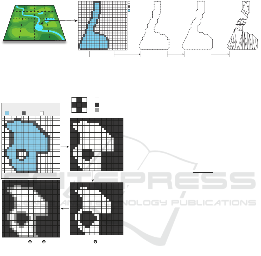
into blocks of fixed size in the CPU. Fig. 2 presents a
visual overview of the process discussed below.
The process begins by selecting a block and invok-
ing a Buffering (Sec. 4) process. A texture is used,
in which each pixel covers a specific area within the
block. On the GPU, each pixel is processed indepen-
dently and filled according to its position relative to
the waterbodies, being classified as Inside, Outside or
Border pixel.
The texture generated in the previous step is re-
trieved to the CPU. It goes through a Vectorization
(Sec. 5) process to extract the previously filled pix-
els, where Border pixels form a circular path that is
traversed to generate the final polygons representing
the waterbodies. This process works based on a graph
data structure with a backtracking-like algorithm. Af-
terward, these polygons are then Simplified (Sec. 6)
using a modified version of the Douglas-Peucker al-
gorithm (Douglas and Peucker, 1973), which is a so-
lution to simplify a curve composed of line segments
to a similar curve with fewer points.
The extracted polygons are Triangulated (Sec. 7)
using a constrained Delaunay triangulation algorithm
(Chew, 1989), generating the mesh for a block of the
scenario, which is saved in the disk.
4 TEXTURE GENERATION
A texture represents a discretization of a continuous
block of the scenario, where each pixel represents a
small portion of a block. A pixel size covering a spe-
cific area inside the block and a portion of the scenario
is selected. The texture size is then calculated by:
TextureSize = BlockSize/PixelSize (1)
An extra padding of 1 pixel is added on Eq. (1),
ensuring the correct connection between blocks.
The PixelSize value directly relates to the final
mesh quality and the memory and time resources
spent on the texture generation. If a small pixel size
is used, the final mesh is closer to a geometric so-
lution, resulting in a more accurate representation in
exchange of adding more vertices. Albeit the more
refined result, the memory use increases due to the
large texture needed to cover the block area. A larger
pixel size will result in a coarser mesh, where small
details can be lost due to the pixel covering a large
scenario area, but the time and memory cost will be
much lower. Usually, the chosen PixelSize is kept be-
tween a range of 0.5 and 1 meter, to allow a good ge-
ometric result and to keep the memory cost in a good
range. Larger or smaller PixelSize will lead to a worse
mesh or a higher memory cost, respectively.
Using the information previously set, the genera-
tion consists on taking the distance of every pixel to
the closest river or lake edge, using the acceleration
structures on the GPU. The used accelerated struc-
tures are composed of a linear spatial hash (Pozzer
et al., 2014) for subdividing the terrain and allowing
fast access to the polyline data, and a quadtree struc-
ture (Engel et al., 2016) representing the polygons,
allowing fast point-in-polygon queries. According to
the distance, pixels are classified in three different
types (Fig. 2):
• Outside, pixels outside a river ∧ lake;
• Inside, pixels fully contained in the river ∨ lake;
• Border, pixels as border to a river ⊕ lake.
where ∧ denotes AND operation; ∨ inclusive OR;
and, ⊕ exclusive OR.
Pixels belonging to the texture border, classified
as Inside, are overwritten as Border pixels. This spe-
cial case is necessary to guarantee a correct junction
A Raster-based Approach for Waterbodies Mesh Generation
145
Block
Inside
Outside
Border
Buffering
Vectorization
Simplification
Triangulation
Scenario
Figure 2: Overview of the algorithm execution.
between blocks, without T-vertex, as well to ensure a
circular path through the Border pixels, to traverse the
texture and extract the polygons.
(A’ B)
Outside
Border
Inside
Foreground
Background
Eroded Border
A
A’
A’ B
A’
V =
B
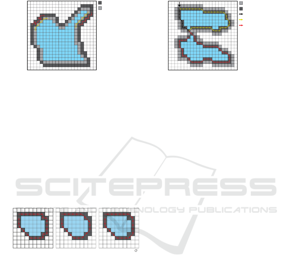
Input Block
Figure 3: A visual description of the erosion process. B
represents the structuring element, A the generated texture.
A’ is the A texture without its borders. The subsequent fig-
ures indicated by the arrows are a visual representation of
the process. In the last figure, the grey pixels indicate the
eroded border obtained.
Due to the high computational cost of the Vector-
ization step, since the execution time of the algorithm
used to guarantee the correct polygon is directly re-
lated to the number of neighbors to a pixel, an erosion
process, described in Eq. (2) and illustrated on Fig. 3,
is applied to mitigate the number of neighbors.
This process works as follows: Let A represent
the pixel set defined by the generated texture, where
Inside pixels are foreground pixels, and every other
pixel type are background pixels, considering A
0
as
the A pixels set without its borders, represented on
Fig. 3. Let B represent the structuring element of a
3x3 matrix in a cross structure. The resulting texture
is given by:
T = (A
0
B) ⊕ A
0
(2)
where denotes erosion and ⊕ denotes an exclusive
OR operation applied pixel-wise.
The texture T obtained is again padded with the
original borders present in A, generating a polygon
representing an eroded version of the polygon gener-
ated in the previous step.
Due to the erosion process, an offset is applied to
the vertex positions in relation to the initial computed
position. For the rivers, the vertices after the erosion
will have a position of
RiverWidth
2
− PixelSize in rela-
tion to the river polyline. For the polygons, there is an
offset of PixelSize in relation to the original border.
To guarantee that the final vertices will have the
desired position, the RiverWidth is considered as
RiverWidth + (2 ∗ PixelSize). For lakes, instead of
setting pixels that intersect the polygon edges as Bor-
der, pixels at a distance of PixelSize from the edge are
considered.
Fig. 4 presents the difference between the ex-
tracted polygon before and after erosion. It’s possi-
ble to notice that the original borders of the polygon
have more neighbors than needed, leading to errors or
stair-like behavior on the border of the polygon being
extracted.
5 POLYGON EXTRACTION
With the generated texture a vectorization algorithm,
as seen in Fig. 2, is applied, in CPU, to extract the
generated polygons border from the texture. The pro-
cess starts by selecting any Border pixel from the tex-
ture. From this pixel, its neighbors are evaluated, and
the chosen neighbor is selected as the next pixel. This
process occurs until the first selected pixel is reached
again. When a pixel is evaluated, it is set as visited. If
it gets revisited, it is marked to not be chosen again,
avoiding self-intersections in the extracted polygon.
GRAPP 2021 - 16th International Conference on Computer Graphics Theory and Applications
146
Border
Eroded Border
Figure 4: Representation of the difference between the ex-
tracted path on a polygon before and after applying the ero-
sion process. The red arrows represents the ordered pixels
list being extracted as the polygon border, before applying
the erosion, while the yellow arrows represents the path col-
lected after the erosion.
In some cases, as described in Fig. 5, a pixel has
more than one neighbor; this can lead to ambiguity
when extracting the polygon. In such cases, a set of
possible heuristics to select the next pixel from the
neighbor’s list can be defined:
• Closest Distance: The closest pixel to the current
pixel is selected;
• Directional: The most clockwise or counter-
clockwise pixel in relation to the last formed seg-
ment is selected;
• Least Angle: The pixel forming the least angle in
relation to the last formed segment is selected.
Closest Distance Directional Least Angle (Clockwise )
Figure 5: Representation of how the different heuristics deal
with branches in the polygon extraction step. The red line
represents what polygon would be extracted in each heuris-
tic.
An extracted polygon is one that the last extracted
pixel has no more valid neighbors and is inside a de-
fined distance threshold to the first extracted pixel.
The previously defined heuristics present a problem.
If it chooses a wrong pixel, it can lead to the polygon
not being extracted, as seen in Fig. 6. To avoid this, as
it would lead to inconsistencies between the original
river network and the generated mesh, a graph data
structure with a backtracking-like algorithm is intro-
duced to solve this inconsistency. The algorithm runs
as follows:
Path
Possible Path B
Possible Path A
Border
Eroded Border
Figure 6: Representation of a wrong path when extracting
the polygon. The black path represents the extraction until
a branch is found, then the red path represents a wrong path,
while the yellow path is the correct one.
WHILE(!extracted(threshold, current, initial))
neighbours = getNeighbours(current)
IF (neighbours = 0)
IF (extracted(threshold, current, initial))
RETURN generatePolygon(current)
ELSE
neighbours = getVisited(current)
IF (neighbours = 0)
current = backtrack(current)
ENDIF
ENDIF
ELSE
current.neighbours = neighbours
current = getNextNode(current)
ENDIF
ENDWHILE
Given an initial pixel chosen at random, a node
denoted as current is created representing it. Then, all
adjacent pixels are searched to verify if any of them
is valid. If no neighbors are found, a verification is
made to check if the polygon is already extracted. If
not, the algorithm backtracks to the last node that had
more than one neighbor and removes the pixel leading
to the dead-end path from the neighbor’s list. If there
are valid neighbors around the current node, they are
added to the neighbor’s list, and one of the aforemen-
tioned heuristics is applied to find the next node to
be processed. When the initial pixel is reached, the
polygon is saved for the next steps, and the process
starts again since more polygons can be encoded in
the texture.
Contrary to the texture generation, which presents
a high level of parallelism, the polygon collection step
is not trivially parallelizable, since the vertex order
must be kept. Considering this, the process is done
sequentially, and the feature density is a factor that
increases the execution time.
A Raster-based Approach for Waterbodies Mesh Generation
147

6 POLYGON SIMPLIFICATION
Geometric buffering solutions guarantee a minimal
vertex count of the generated polygons. Opposed to
this, our solution produces more vertices than neces-
sary, requiring a simplification to ensure a lower num-
ber of vertices that composes the final polygon geom-
etry, which, in turn, will speed up the rendering. Also,
the fact that any vertex can be removed from the final
simplified polygon presents a problem when dealing
with vertices in the borders of blocks, as removing
these vertices can lead to t-junctions in the generated
mesh between distinct blocks.
As such, an adaptation of the Douglas-Peucker
simplification algorithm is proposed.
The Douglas-Peucker algorithm takes as input an
ordered set of points and a parameter T as a distance
for defining whether a vertex shall belong to the sim-
plified curve or not. The algorithm maintains the first
and last points to be kept and find the farthest point to
the formed line. If the distance from the point to the
line is greater than the distance T , it is added to the
list and the algorithm splits the curve into two sepa-
rate pieces to be processed: The initial point and the
collected point P; and the point P and the final point.
This process occurs until there are no more points at
a distance greater than T .
The modification consists of adding the necessary
vertices in the list of vertices to be kept, together with
the initial and final vertex, at the start of the algo-
rithm execution. There is a need to remove duplicated
points in the algorithm output since the border ver-
tices are not removed from the algorithm input and
are added to the output list at the beginning of the ex-
ecution.
For measuring the simplification amount, Eq. (3)
describes an approximation for the minimal vertex
count that should be achieved.
V =
VertexCount
2 ∗ River
Vertices
+ Lake
Vertices
(3)
The river segments vertex count is duplicated in
the equation since the input polyline is extruded in
both sides to compose the river’s border. As a result,
if V = 1, the minimum number of vertices has been
achieved, values greater than one characterize a ge-
ometry with an excess of vertices.
It is essential to keep a small simplification factor,
as the Douglas-Peucker algorithm is known to gen-
erate polygon self-intersections when using a large
parameter T . A non-self-intersecting algorithm was
proposed by (Wu and Marquez, 2003).
7 TRIANGULATION
The triangulation is the last step. It’s applied after the
polygon simplification step. First, a hole detection al-
gorithm is employed. The bounding box of a polygon
is checked to assert that it is fully contained inside
another polygon bounding box. If the bounding box
is contained, a point in polygon test is done to every
polygon point. If all points are contained inside an-
other polygon, it is set as a hole. This test is executed
to all polygons in the block.
Each polygon and its respective holes, if existent,
are input into a Constrained Delaunay Triangulation
algorithm (Chew, 1989). The triangulation result is a
polygonal mesh corresponding to the borders of the
extruded river and lake data initially fed to the algo-
rithm.
The generated mesh undergoes a mesh simplifica-
tion algorithm (Schroeder et al., 1992),(Heckbert and
Garland, 1999) with vertex-vertex distance criteria.
This process reduces the vertex count even more on
the final mesh, as well as creating seamless junctions
between block borders, which is possible through the
addition of padding to the texture, discussed in sec-
tion 4. The resulting mesh is then saved to disk in the
desired format.
8 RESULTS
The experiments were performed on an AMD
Ryzen 5 3.6 GHz processor, with 16 GB of RAM and
an NVIDIA GeForce GTX 1070 graphics card, with
8 GB VRAM. The proposed architecture was imple-
mented in C# and HLSL languages using the Unity
engine. However, it is a generic solution and can be
implemented in any language.
We run experiments on five real-world datasets
comprised of vector data. The datasets were cho-
sen based on feature density, covered area, and vertex
count. The experiments explore time, memory, and
visual fidelity results; also, total triangle and vertex
count for the resulting polygonal mesh are analyzed.
All results were based on an average time of five ex-
ecutions. The individual information for each dataset
can be seen in Table 1.
8.1 Memory Analysis
First, a static memory consumption analysis of the so-
lution is made. Due to the block approach, the analy-
sis is done considering a single block of the scenario.
For implementation purposes, we use an integer
texture for storing an index pointing to a position in-
GRAPP 2021 - 16th International Conference on Computer Graphics Theory and Applications
148
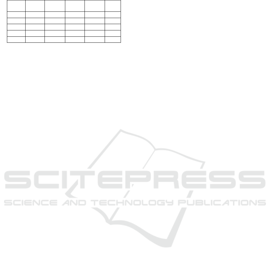
Table 1: Test Datasets.
Dataset
River
Vertices
River
Features
Lake
Vertices
Lake
Features Area
a
L1 34923 1059 8122 130 1980
L2 90741 2939 3376 14 729
L3 279354 24922 41520 731 1485
L4 281743 5208 2266 9 1485
L5 641022 44825 83867 1519 36852
a
Area is represented in KM².
side a buffer containing the vertex data. This buffer
contains two float values for storing the vertex posi-
tion, an integer storing a pointer to the texture pixel
representing this vertex, and 1 byte for storing addi-
tional info. As such, the V-RAM cost can be calcu-
lated as defined in Eq. (4).
V RAM
Usage
= (TextureSize
2
× 4) + (α ∗Vertex
Cost
)
(4)
where α denotes the variable buffer size, Vertex
Cost
is the individual memory cost for each vertex and
TextureSize is calculated as defined in Eq. (1).
In CPU, the memory cost is calculated as the pre-
viously estimated V-RAM usage plus the individual
graph node memory cost times the vertex buffer size.
The memory cost is relevant because it defines
how large a block can be and what resolution can be
used to represent a portion of the virtual scenario. For
example, a 100x100 kilometers scenario, with 4096
meters per block and a pixel size of 0.5 meters, will
have a total of 625 blocks, considering α as 65000
vertices, where each block requires 256 MB of mem-
ory.
Since each block is individually processed, an op-
timization based on CPU parallelization can be em-
ployed to process more than one block in parallel.
As such, the parallelization amount is defined by how
many blocks can be fit into the memory and the num-
ber of cores available.
8.2 Time Performance Analysis
Table 2 presents the performance of the solution. The
test suite settings were: Block size of 4096 meters,
pixel size of 0.5 meters, Closest Distance heuristics,
and simplification using T = 0.25 meters.
It’s possible to notice that the Texture Genera-
tion process time is linear, highly dependent on the
scenario area. For example, the datasets L3 and L4
present the same size, with similar texture genera-
tion times; or, between L2 and L3, where L3 area is
roughly double the size of L2 and presents a propor-
tional time cost. Finally, L5 presents a larger texture
generation time than others due to its larger area.
Since this step happens in a highly parallel fash-
ion, the acceleration structures avoid that the fea-
ture density increase drastically the texture generation
time, as well as the fact that each pixel is processed
independently.
The polygon extraction step is executed on the
CPU and is more dependent on feature density than
the block size. L3, having the same area as L4, takes
3.11 more time on the polygon extraction than L4.
We can make a relation between the time growth
and the feature density difference between datasets.
While L3 has 1.13 more vertices than L4, which
would not justify the difference in time, the more sig-
nificant difference is in the number of river and lake
features. This means that L3 has a higher density of
features per block, leading to a higher number of in-
tersections between different rivers and lakes, and a
greater number of cases where the backtracking algo-
rithm may execute.
L5 has the expected execution time, being the
largest dataset, indicating a growth based on the num-
ber of blocks and area size. At the same time, it is less
affected by the increase in execution time due to the
feature density.
The Polygon Simplification, Hole Detection and
Triangulation steps present execution times directly
related to the polygons amount extracted on the
Polygon Extraction step and the total vertex count.
Datasets with high vertices count perform worse than
others with fewer vertices, as seen in L5 and L3 com-
pared to the other datasets. L3 fares even worse than
L5 due to the smaller area and the high vertex count,
leading to a bigger vertices/block count. The high
number of lake vertices also contributes to the slow
execution, as usually only lakes contain holes.
In L4 and L3, there is a significant difference in
execution time besides both datasets having a small
difference in vertex count. The lake vertices count in
L3 is 18.32 times bigger compared to L4, justifying
the difference in time.
8.3 Simplification Impact Analysis
Table 3 presents five results of vertices count on L3
and L2, using different simplification factors. It’s pos-
sible to conclude that a suitable simplification param-
eter is achieved when T equals the pixel size value,
as larger simplification values do not reduce much
the total vertex count and can lead to polygon self-
intersection, as discussed in Sec. 6. Small simplifica-
tions should be avoided; the results indicate that the
time is exponentially larger as the simplification fac-
tor is low or nonexistent. Also, high vertices lead to
low performance when rendering the mesh.
The simplification factor is directly related to the
Hole Detection and Triangulation steps. The time
A Raster-based Approach for Waterbodies Mesh Generation
149
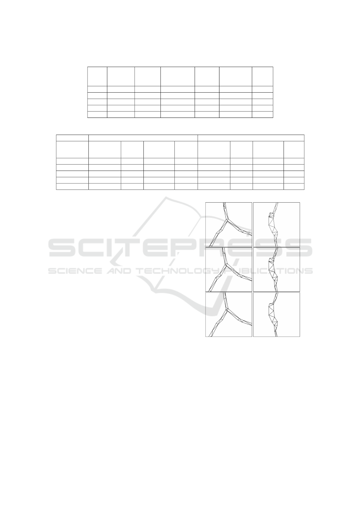
Table 2: Datasets Performance.
Dataset
Texture
Generation
Time
Polygon
Collection
Time
Polygon
Simplification
Time
Hole
Detection
Time
Triangulation
Time
Total
Time
L1 16.95 6.41 22.76 17.37 13.73 77.24
L2 5.66 9.06 32.69 134.65 22.64 204.72
L3 11.83 54.35 146.57 3344.83 111.80 3669.39
L4 10.25 17.46 59.49 125.42 41.48 254.12
L5 244.73 229.71 945.62 1828.28 564.40 3812.75
a
All times presented are in seconds.
Table 3: Simplification Results.
Datasets L1 L2
Simplification
Amount
Simplification
Time
Hole
Detection
Time
Triangulation
Time
Vertex
Count
Simplification
Time
Hole
Detection
Time
Triangulation
Time
Vertex
Count
0 0 48917.26 617.16 26012450 0 2379.94 134.24 6189517
0.25 147.07 3137.94 113.04 6537075 32.65 137.86 22.87 1486307
0.5 94.19 55.25 9.37 882699 22.1 2.61 1.72 185680
0.75 91.71 46.24 8.22 809815 21.53 1.89 1.41 159763
1 90.78 48.57 7.88 775492 21.02 1.49 1.19 140686
a
All times presented are in seconds.
with a simplification equal to the pixel’s size pre-
sented a reduction of almost a thousand times in the
execution time for L3 and L2 Hole Detection step, in-
dicating the importance of applying a simplification
algorithm.
The simplification amount, considering the 0.5
simplification parameter, as calculated in Eq. (3), for
L3 was V = 1.47, which is a good result considering
the raster-based generation. For L2, it was V = 1.00,
indicating an optimal simplification.
8.4 Visual Results
Concerning the visual results, Fig. 7 presents a wire-
frame representation of the generated meshes using a
pixel size of 0.5, 1, and 2 meters. The visual differ-
ence is perceptible when larger pixel sizes are used,
mainly in the junctions, where they tend to be rougher.
The lake part of the mesh also suffered a loss of detail
with larger pixel sizes.
Fig. 8 shows the mesh laid on top of the terrain,
allowing the analysis of the obtained triangulation,
which presented satisfactory results.
Fig. 9 presents the generated mesh rendered onto
the terrain. Two different water shaders are being ap-
plied in Fig. 9, showing that our resulting mesh can
be used for an accurate representation of the water-
bodies.
Figure 7: Representation of the generated mesh. In this
case, a river-river (left) and river-lake (right) junctions are
presented. From top to bottom, the pixel size used was: 0.5,
1.0, 2.0 meters.
9 CONCLUSION
We presented a solution for generating waterbody
meshes for arbitrarily sized scenarios with a straight-
forward approach based on buffering and dissolve
techniques, using a raster-based approach to simplify
the process and allow a simple treatment of junctions
between the input data.
GRAPP 2021 - 16th International Conference on Computer Graphics Theory and Applications
150
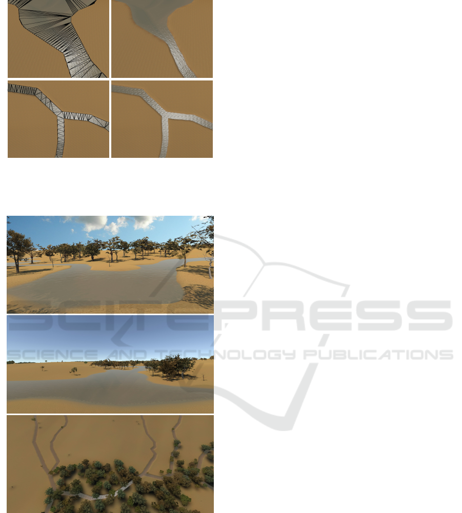
Figure 8: Depiction of a river-river (bottom) and a river-lake
(top) junction, laid onto the terrain. In the left images, for
a better viewing of the wireframe, the water plane has been
lift above the terrain.
Figure 9: Representation of the generated mesh laid onto
the terrain with a water shader applied.
Our results show that the proposed solution is
scalable and allows the mesh generation for large sce-
narios, having an execution time directly related to the
scenario size and feature density. The solution’s bot-
tleneck is the Hole Detection algorithm used, which
is not the primary concern of this work.
The Polygon Extraction and Texture Generation
steps, which were the main concerns of this work,
together with the Triangulation step, presented satis-
factory results in relation to time and output results.
Utilizing a texture to create the buffered lines dis-
solved with the polygons allowed the treatment of
both rivers and lakes interchangeably, eliminating the
need to create different algorithms for each type of
junctions, simplifying the polygon generation. The
quality of the exported mesh and its vertex count is
also satisfactory when small pixel sizes are used to-
gether with a good simplification factor, as shown in
Fig. 7 and Fig. 9. The block approach allows the
solution to work with large scenarios and enables the
use of a parallelization algorithm where each block is
independently processed, leading to further optimiza-
tions on the solution.
For future work, we propose:
• Study better and more stable methods of triangu-
lation, and discuss the relation between quality
and performance of the triangulation in the con-
text of the proposed solution;
• Use other type of georeferenced data, like eleva-
tion maps, to generate a more accurate and de-
tailed mesh;
• Parallelize each block processing, in a pipeline
fashion;
• Implement a faster and more robust Hole Detec-
tion algorithm;
• Implement a non-self-intersecting Douglas-
Peucker algorithm, allowing greater levels of
simplification;
• Analyse and attempt to extend the solution to
other similar problems, such as mesh genera-
tion for roads, which present the same geometry
generation issue, allowing to generate highway
meshes with seamless junctions between roads
and bridges.
ACKNOWLEDGEMENTS
We thank the Brazilian Army and its Prg EE AS-
TROS 2020 for the financial support through the SIS-
ASTROS project.
REFERENCES
Bhatia, S., Vira, V., Choksi, D., and Venkatachalam, P.
(2013). An algorithm for generating geometric buffers
for vector feature layers. Geo-Spatial Information Sci-
ence, 16(2):130–138.
A Raster-based Approach for Waterbodies Mesh Generation
151

Chew, L. P. (1989). Constrained delaunay triangulations.
Algorithmica, 4(1-4):97–108.
Dong, P., Yang, C., Rui, X., Zhang, L., and Cheng, Q.
(2003). An effective buffer generation method in
gis. In IGARSS 2003. 2003 IEEE International Geo-
science and Remote Sensing Symposium. Proceedings
(IEEE Cat. No. 03CH37477), volume 6, pages 3706–
3708. Ieee.
Douglas, D. H. and Peucker, T. K. (1973). Algorithms for
the reduction of the number of points required to rep-
resent a digitized line or its caricature. Cartographica:
the international journal for geographic information
and geovisualization, 10(2):112–122.
Engel, T. A., Frasson, A., and Pozzer, C. T. (2016). Op-
timizing tree distribution in virtual scenarios from
vector data. Proceedings of Brazilian Sympo-
sium on Computer Games and Digital Entertainment
(SBGames).
Engel, T. A. and Pozzer, C. T. (2016). Shape2river: a tool
to generate river networks from vector data. Proceed-
ings of Brazilian Symposium on Computer Games and
Digital Entertainment (SBGames).
Fan, J., He, H., Hu, T., Li, G., Qin, L., and Zhou, Y.
(2018). Rasterization computing-based parallel vec-
tor polygon overlay analysis algorithms using openmp
and mpi. IEEE Access, 6:21427–21441.
Heckbert, P. S. and Garland, M. (1999). Optimal triangu-
lation and quadric-based surface simplification. Com-
putational Geometry, 14(1-3):49–65.
Kryachko, Y. (2005). Using vertex texture displacement for
realistic water rendering. GPU gems, 2:283–294.
Ma, M., Wu, Y., Luo, W., Chen, L., Li, J., and Jing, N.
(2018). Hibuffer: buffer analysis of 10-million-scale
spatial data in real time. ISPRS International Journal
of Geo-Information, 7(12):467.
Pozzer, C. T., Pahins, C., Heldal, I., Mellin, J., and Gustavs-
son, P. (2014). A hash table construction algorithm for
spatial hashing based on linear memory. In Proceed-
ings of the 11th Conference on Advances in Computer
Entertainment Technology, pages 1–4.
Schroeder, W. J., Zarge, J. A., and Lorensen, W. E. (1992).
Decimation of triangle meshes. In Proceedings of the
19th annual conference on Computer graphics and in-
teractive techniques, pages 65–70.
Shen, J., Chen, L., Wu, Y., and Jing, N. (2018). Approach
to accelerating dissolved vector buffer generation in
distributed in-memory cluster architecture. ISPRS In-
ternational Journal of Geo-Information, 7(1):26.
Wu, S.-T. and Marquez, M. R. G. (2003). A non-
self-intersection douglas-peucker algorithm. In 16th
Brazilian symposium on computer graphics and Im-
age Processing (SIBGRAPI 2003), pages 60–66.
IEEE.
Yu, Q., Neyret, F., Bruneton, E., and Holzschuch, N. (2009).
Scalable real-time animation of rivers. Computer
Graphics Forum (Proceedings of Eurographics 2009),
28(2). to appear.
GRAPP 2021 - 16th International Conference on Computer Graphics Theory and Applications
152
