FLIC: Fast Lidar Image Clustering

Frederik Hasecke

1,2 a

, Lukas Hahn

1,2,∗ b

and Anton Kummert

1 c

University of Wuppertal, Faculty of Electrical Engineering, Wuppertal, Germany

Aptiv, Wuppertal, Germany

Keywords:

Clustering, Dimensionality Reduction, LiDAR.

Abstract:

In this work, we propose an algorithmic approach for real-time instance segmentation of Lidar sensor data. We

show how our method uses the underlying way of data acquisition to retain three-dimensional measurement

information, while being narrowed down to a two-dimensional binary representation for fast computation.

Doing so, we reframe the three-dimensional clustering problem to a two-dimensional connected-component

labelling task. We further introduce what we call Map Connections, to make our approach robust against over-

segmenting instances and improve assignment in cases of partial occlusions. Through detailed evaluation on

public data and comparison with established methods, we show that these aspects improve the segmentation

quality beyond the results offered by other three-dimensional cluster mechanisms. Our algorithm can run at

up to 165 Hz on a 64 channel Velodyne Lidar dataset on a single CPU core.

1 INTRODUCTION

Lidar sensors have been introduced in an ever grow-

ing number of different driver assistance systems to

automotive series production in recent years and are

considered an important building block for the prac-

tical realisation of autonomous driving. Precise seg-

mentation of object instances is an important infor-

mation for a variety of applications ranging from on-

line object detection to ofﬂine computer-aided data la-

belling. Lidar sensor data is usually represented as

a three-dimensional point cloud in Cartesian coordi-

nates. Hence it makes sense to consider clustering al-

gorithms to fulﬁl the task of object segmentation for

this type of sensor. This work presents a Lidar point

cloud segmentation approach, which provides a high

level of accuracy in point cloud segmentation, while

being able to run in real time, faster than the sensor

recording frequencies at a constant rate with very lit-

tle ﬂuctuation independent of the scene’s context. We

https://orcid.org/0000-0002-6724-5649

https://orcid.org/0000-0003-0290-0371

https://orcid.org/0000-0002-0282-5087

∗

This work is a result of the research project @CITY

Automated Cars and Intelligent Trafﬁc in the City. The

project is supported by the Federal Ministry for Economic

Affairs and Energy (BMWi), based on a decision taken by

the German Bundestag. The author is solely responsible for

the content of this publication.

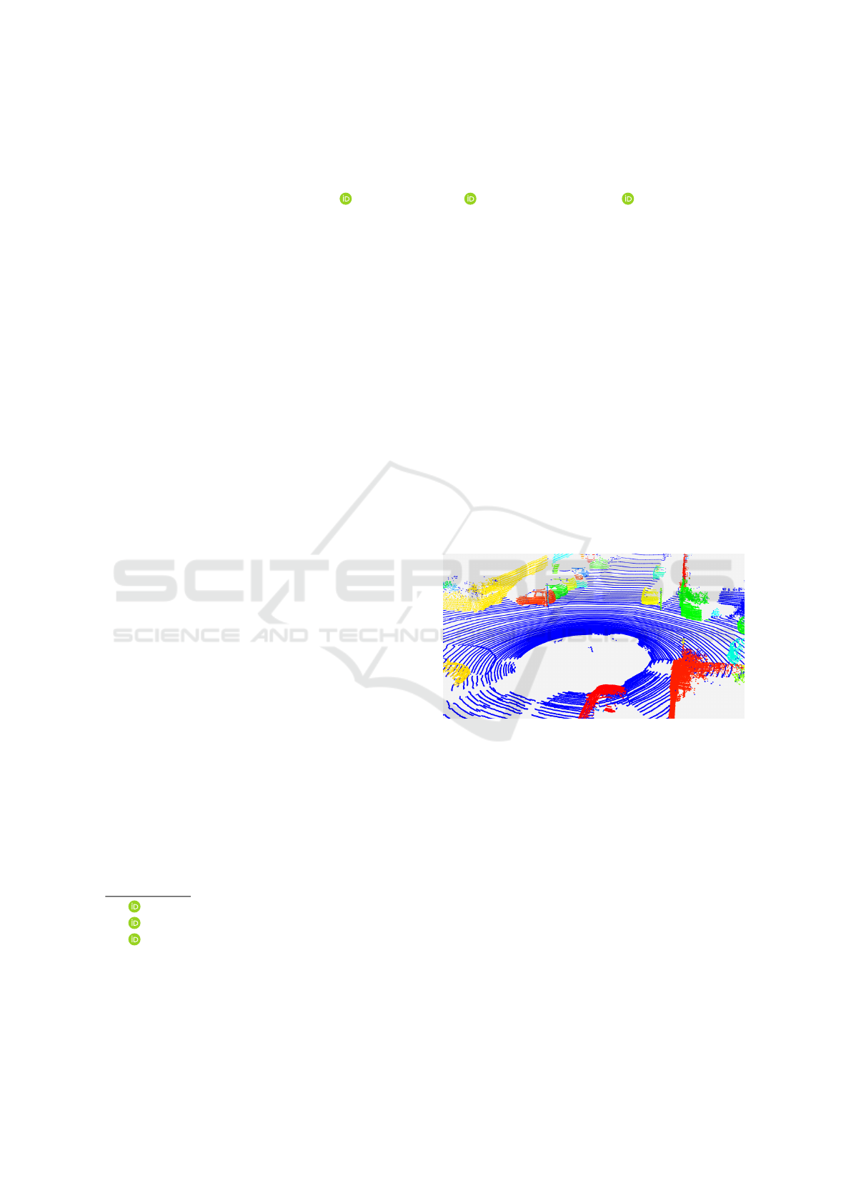
Figure 1: Three-dimensional point cloud with clustered

points. Every Instance is assigned a random colour.

do so by avoiding the creation of a three-dimensional

point cloud from the range measurements provided by

the Lidar scanner and work directly on the laser range

values of the sensor. If not available, the computations

can be applied to a spherical range image projection

of the three-dimensional point cloud and projected

back to the point cloud as demonstrated in Figure 1.

This approach circumvents the problem of sparsity in

the point cloud by forcing a two-dimensional neigh-

bourhood on each measurement and thus offers the

advantage of working with dense, two-dimensional

data with clearly deﬁned neighbourhood relationships

between adjacent measurements. A Python imple-

mentation of our approach runs in real time on a single

Intel



Core

i7-6820HQ CPU @ 2.70 GHz core at

a frame rate of up to 165 Hz.

Hasecke, F., Hahn, L. and Kummer t, A.

FLIC: Fast Lidar Image Clustering.

DOI: 10.5220/0010193700250035

In Proceedings of the 10th International Conference on Pattern Recognition Applications and Methods (ICPRAM 2021), pages 25-35

ISBN: 978-989-758-486-2

2 RELATED WORK

There is a large number of previous works on Lidar

instance segmentation especially of, but not limited

to, automotive applications. The main focus of most

clustering approaches is on improving segmentation

accuracy and execution time. Most of these separate

objects in the three-dimensional space, result in high

accuracy but comparatively long runtime. Notable ex-

amples are the DBSCAN (Ester et al., 1996), Mean

Shift (Fukunaga and Hostetler, 1975) (Comaniciu and

Meer, 2002) and OPTICS (Ankerst et al., 1999) algo-

rithm.

Other approaches use voxelization to reduce the

complexity of the point cloud and ﬁnd clusters in the

representation (Himmelsbach et al., 2010) or apply

bird’s eye view projection coupled with the height in-

formation to separate overlapping objects (Korchev

et al., 2013).

(Moosmann et al., 2009) proposed the use of a

local convexity criterion on the spanned surface of

three-dimensional Lidar points in a graph-based ap-

proach. Based on this metric, (Bogoslavskyi and

Stachniss, 2016) used a similar criterion - the spanned

angle between adjacent Lidar measurements in rela-

tion to the Lidar sensor origin - to deﬁne the convex-

ity of the range image surface as a measure to seg-

ment objects. They further utilise the neighbourhood

conditions in the range image to achieve the fastest

execution time to date. (Zermas et al., 2017) exploit

the same relationship in scan lines of Lidar sensors to

ﬁnd break points in each line and merge the separate

lines of channels into three-dimensional objects in a

subsequent step.

Other current methods use machine learning di-

rectly on three-dimensional point clouds (Lahoud

et al., 2019) (Zhang et al., 2020) (Yang et al., 2019),

projections into a camera image (Wang et al., 2019a),

or on spherical projections of Lidar points in the range

image space (Wang et al., 2019b), to segment object

instances in point clouds. These results look very

promising in some cases, but suffer from a longer run-

time, which currently prevents application on embed-

ded automotive hardware.

Related research areas that need to be mentioned

at this point are the semantic segmentation and even

more so the panoptic segmentation of Lidar data. The

dataset “SemanticKITTI”(Behley et al., 2019), which

we use to evaluate our method in 4.2, has advanced

a number of new algorithms in the area of seman-

tic segmentation (Kochanov et al., 2020) (Zhou et al.,

2020) (Zhang et al., a). The task is concerned with the

classiﬁcation of each Lidar point. Leading algorithms

have achieved great performance on assigning a class

label and some are even real-time capable on a sin-

gle GPU (Tang et al., 2020) (Gerdzhev et al., 2020)

(Cortinhal et al., 2020). The difference to instance

segmentation is the separation of instances. The se-

mantic segmentation does not differentiate between

multiple objects, but assigns the same label to each in-

stance of the same class. The panoptic segmentation

is the combination of the semantic and the instance

segmentation. (Milioto et al., 2020) even manage to

reach real-time capability on a single GPU with a run-

time of 85 ms by jointly segmenting the instances and

the class.

Our method is concerned with the separation of in-

stances independently of the class labels. We base our

approach on the works of Bogoslavskyi and Stachniss

(Bogoslavskyi and Stachniss, 2016) as well as general

three-dimensional Euclidean algorithms (Ester et al.,

1996) (Fukunaga and Hostetler, 1975) (Comaniciu

and Meer, 2002) (Ankerst et al., 1999). We com-

bine the fast execution time of range image clustering

with the precise segmentation of distance thresholds

to connect and separate Lidar points.

3 METHODS

The raw data from Lidar sensors is usually provided

as a list of range measurements, each coupled with

a number relating to the channel and the lateral po-

sition. The two values correspond to the y- and x-

position of the measurements in the range image.

This can also be used to create a three-dimensional

representation of the measurements, but doing so

will increase the computation time for the proposed

method. Therefore, we work directly on the raw two-

dimensional representation.

3.1 Ground Extraction

For object segmentation, we assume that the Lidar is

a part of a ground-based vehicle. Based on this as-

sumption, we want to extract and ignore the points

belonging to the ground plane from the segmentation.

This will prevent the algorithm from connecting two

instances via this plane. Here, a simple height based

threshold is not sufﬁcient, as the road surface itself

can be uneven. Pitching and rolling of the ego vehicle

can also inﬂuence the way the ground is perceived in

the sensor data. Since we have detailed information

about the Lidar sensor itself, we can use the angle po-

sition of each given channel to determine the angle in

which the laser beam would hit the surface. We use

this information to exclude all range image values be-

longing to a horizontal plane below a certain height.

ICPRAM 2021 - 10th International Conference on Pattern Recognition Applications and Methods

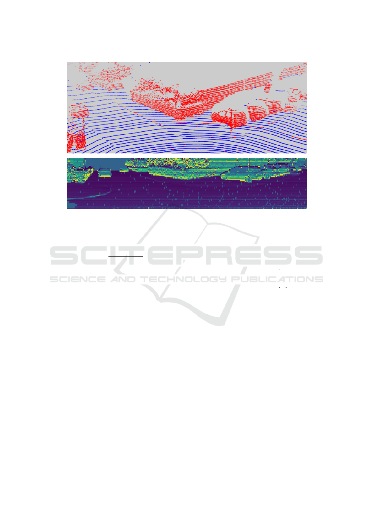
Figure 2: Top: Ground segmentation; Blue points represent ground points, red points are not part of the ground.

Bottom: Angle image used to ﬁnd horizontal surfaces for the ground segmentation.

To do so, we compare each cell of the range image

with the neighbouring one above using the equation

β = arctan (

· sin α

− d

· cos α

), (1)

in which the selected cell value is d

, the one above

the cell is d

corresponding to the respective depth

measurement and α is the angle between the two mea-

surements.

As a result, we obtain the image shown in Figure

2 representing the angle values of the Lidar beam in

relation to the point cloud surface spanned between

the current Lidar measurement and the measurement

of the Lidar channel below, (see Figure 3). Using a

lookup table of the channel angles δ

with respect to

the channel r, we exclude all range image cells that

span a horizontal surface up to a certain threshold an-

gle θ of ±10

◦

to a full horizontal surface.

To speed up the computation we change the θ

threshold to the tangent of θ to directly compare the

tangent of β. We therefore remove the arctan from the

equation for β, as it is computationally expensive and

can not easily be provided as a lookup table due to

the two ﬂoat variables d

and d

. We also provide

the sine and cosine of α as constant pre-calculated

values. The proper handling of the quadrants of the

Euclidean plane usually requires the atan2 function

as opposed to the arctan (and therefore the tangent)

(Bogoslavskyi and Stachniss, 2016). We circumvent

this restriction as the provided depth measurements

are always positive or zero, any zero value is automat-

ically removed as ground/invalid value. These pre-

calculations change the equation for the horizontal

plane estimation to a set of multiplications and each

one division and subtraction:

tan(β) =

Constant

}|{

sinα

− d

· cosα

|{z}

Constant

. (2)

This method rejects all horizontal surfaces. To pre-

vent excessive removal of valid measurements from

elevated horizontal surfaces such as car roofs or

hoods, we use a height image, in which the range val-

ues are replaced by the Cartesian z-coordinate in re-

lation to the ego vehicle. We use this image to keep

all horizontal surfaces above a certain height, in the

above case, the line from the wheel position of the ego

vehicle to the maximum possible elevation spanned

by the 10

◦

slope threshold. A comparable metric has

been described by Chu et al. (Chu et al., 2017) al-

though with relative height thresholds, we have de-

cided to use absolute values to reduce the computa-

tion time. Figure 3, top, depicts the relationship of

the channel angles δ

(angle in relation to the hori-

zontal 0

◦

line) to the surface angles β

(angle of the

tangent of two neighbouring measurements and the

sensor origin).

FLIC: Fast Lidar Image Clustering

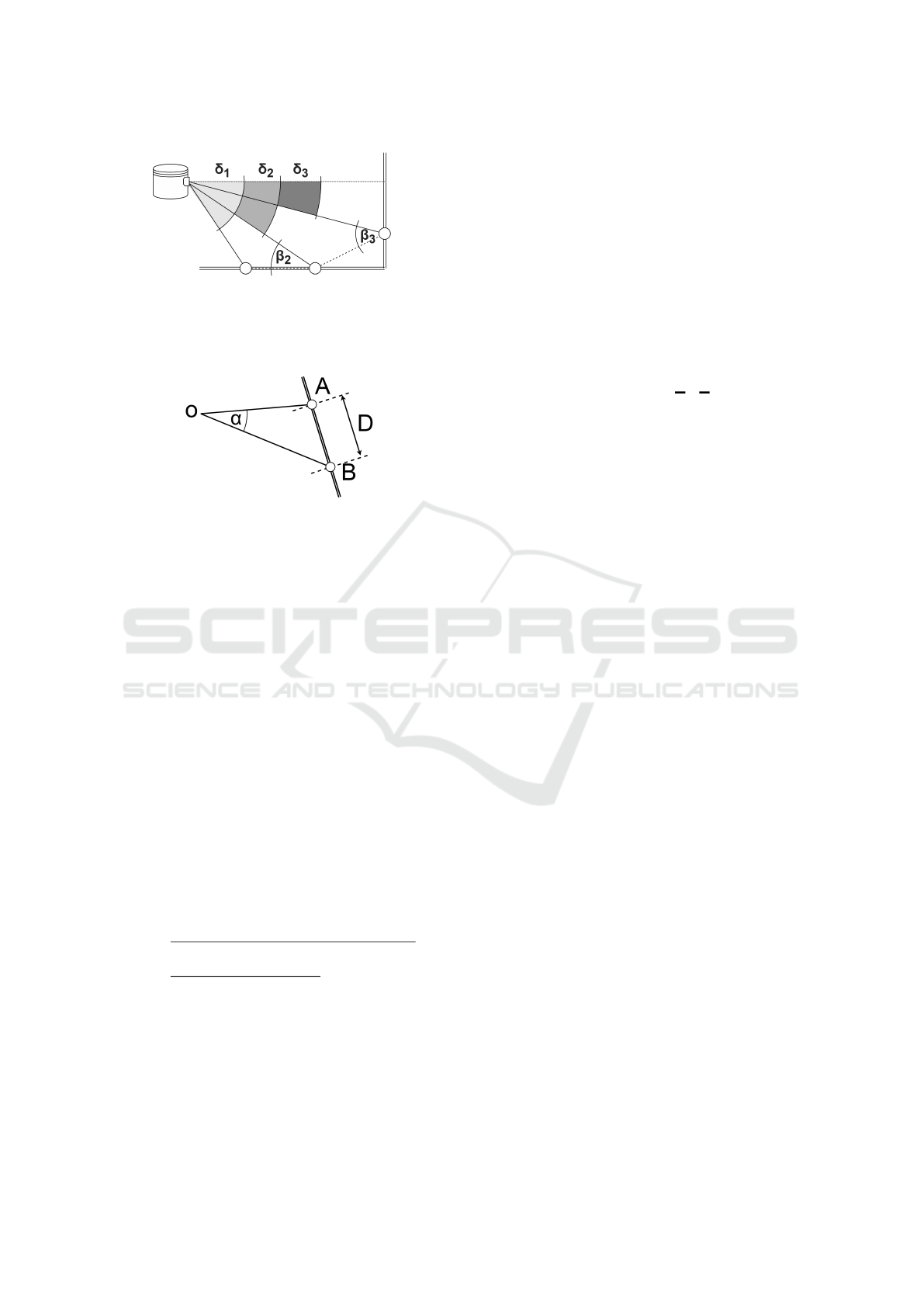
(a) The angle measurement of Lidar points in the

vertical direction is used to deﬁne a horizontal ori-

entation for the ground plane extraction. (Note

that there is not β

, as the ﬁrst Lidar channel has

no previous channel, we therefore extend β

to the

ﬁrst channel.)

(b) With the Lidar Sensor in O, the lines OA

and OB show two neighbouring distance measure-

ments. The distance between the two measure-

ments is calculated using the spanned angle α be-

tween the points.

Figure 3: Trigonometric relationships used in the ground

segmentation (a) and the cluster separation (b).

3.2 Clustering

We use a systematic approach to create an object

instance segmentation for Lidar sensor data through

clustering in the image space of the range image. This

approach relies on the removal of the Lidar measure-

ments belonging to the ground plane from the range

image. Inspired by the work of Bogoslavskyi and

Stachniss (Bogoslavskyi and Stachniss, 2016), we ex-

ploit the neighbourhood relationship of adjacent mea-

surements in the range image. As visualised in the

bottom illustration of Figure 3, we compare the given

range values ||OA|| and ||OB|| for each pair of Li-

dar measurements. We apply the cosine law to calcu-

late the Euclidean distance D in the three-dimensional

space using the two-dimensional range image:

D =

||OA||

+ ||OB||

− 2||OA|| · ||OB||cosα

+ d

− 2 · d

· d

cosα.

(3)

The α angle between adjacent Lidar measurements is

required for the calculation and is usually provided

by the manufacturer of the Lidar sensor for both the

horizontal and vertical direction. Using the physi-

cal distance between two measured points, we de-

ﬁne a threshold value between those, which are close

enough together to belong to the same object, or too

far apart to be considered neighbours on the same ob-

ject. The distance of neighbouring points on a given

object is in general relatively close. The distances

of those points in the range image from two sepa-

rate objects are substantially larger. By exclusively

using variables which are given by the range measure-

ments and reducing the computational effort by pre-

calculating the cosine of the given angles, we reduce

the calculation of the squared Euclidean distance to a

total of four scalar multiplications, an addition and a

subtraction:

= d

· d

+ d

· d

− 2 · cos α

| {z }

Constant

·d

· d

. (4)

These efﬁcient operations are decreasing the runtime

on embedded hardware.

With the calculated threshold between each mea-

surement, we are able to connect all Lidar points in

the range image into separate clusters and background

points. With the use of the Euclidean distance as a

threshold value, we provide a single parameter im-

plementation with a clear physical meaning, which is

adaptable to different sensors.

We reached a good performance with a threshold

of 0.8 metres as the limit for the connections between

two points. This threshold theoretically enables the

clustering of three-dimensional objects with e.g. a

Velodyne HDL-64E up to 114.59 metres before the

measured points are too far apart on a vertical surface.

Horizontally connected components can, in theory, be

detected up to a distance of 509.3 metres which is

more than four times the reliable range for vehicles

of 120 metres, deﬁned by the manufacturer.

3.2.1 Connected-component Labelling

Our approach exploits the vectorised nature of the

range image to apply operations used in image pro-

cessing for different purposes. Speciﬁcally, we

redeﬁne the three-dimensional Euclidean clustering

to a two-dimensional connected-component labelling

(CCL) problem. To do so, we create two virtual

copies of the range image and shift one copy over

the x axis and the other one over the y axis. These

shifted images enable us to stack all three images on

a third axis and compare every value with its vertical

and horizontal neighbour over the whole multidimen-

sional array. Thus by using Equation 4 on this image

we calculate the three-dimensional distance between

each point and his vertical and horizontal neighbour-

ing measurement. After applying the threshold on the

resulting distance values calculated for each measure-

ment and its direct neighbourhood, we end up with

ICPRAM 2021 - 10th International Conference on Pattern Recognition Applications and Methods

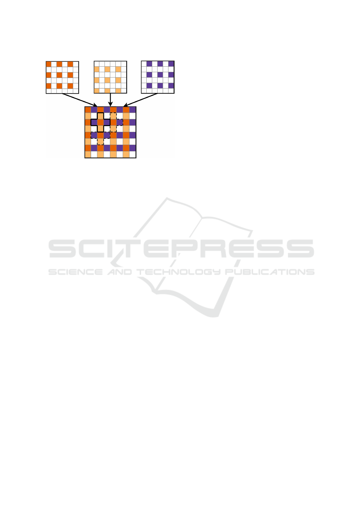
Figure 4: Combination of deﬁned image representations for

instance segmentation. The red squares represent the binary

value of present Lidar measurements, the yellow and blue

squares represent the horizontal and vertical connections of

these measurements respectively.

the original range image and two binary images rep-

resenting the connection or separation between two

points in the range image. The range image is now re-

duced to a binary image representing the presence and

absence of Lidar measurements for the corresponding

pixels in the image.

The three created binary images contain all the

required information to segment the Lidar measure-

ments of the whole frame into clusters and back-

ground points. For this, we utilise a simple and

efﬁcient image processing algorithm; connected-

component labelling. The 4-connected pixel connec-

tivity, also known as von Neumann neighbourhood

(Toffoli and Margolus, 1987), is deﬁned as a two-

dimensional square lattice composed of a central cell

and its four adjacent cells. To apply the pixel connec-

tivity to our data, we combine the binary Lidar mea-

surements with the binary threshold images of the dis-

tances between Lidar points. By arranging these three

images as shown in Figure 4, we are able to apply

CCL algorithms with a 4-connectivity on the resulting

image to label each island of interconnected measure-

ments as a different cluster. The resulting segmented

image is now subsampled to the original range im-

age. Thus we provide the three-dimensional cluster

labels directly from the connected-component image,

as each pixel corresponds to a given Lidar point in the

three-dimensional point cloud.

There is a multitude of CPU-based implemen-

tations for CCL problems most common are the

”one component at a time” (AbuBaker et al., 2007)

and the Two-pass algorithm (Hoshen and Kopelman,

1976). We have decided to use the ﬁrst method

in the straight-forward implementation of the scipy

library ”label” for n-dimensional images (Virtanen

et al., 2020), as it provides a fast cython based func-

tion. More recent CCL algorithms make use of GPUs

by applying the labels in parallel (Hennequin et al.,

2018) (Allegretti et al., 2019). This can be a very

promising approach, as all previous processing steps

in this work are applied to rasterised images and can

be directly computed in parallel on a GPU. We have

not attempted this approach, as our goal is a real-time

application for CPU-based automotive hardware.

In a subsequent step we apply a threshold on the

labelled clusters for objects below a certain number of

Lidar measurements to reduce false clusters resulting

from noise in the sensor, in our case we decided on

a minimum of 100 points to be considered a cluster

candidate, as our objects of interest are cars, pedestri-

ans and other road users. Lower thresholds are rec-

ommended to include static objects such as poles and

debris on the road.

We have thus segmented the measurements into

connected components of separate objects and non-

segmented points, which correspond to the ground

plane and background noise.

3.2.2 Map Connections

Segmentation algorithms are prone to under- and

over-segmentation, due to the characteristics of Lidar

sensors; namely the sparsity (especially in vertical di-

rection) and missing measurements resulting from de-

ﬂected laser beams, which have no remission value

back to the sensor. Missing values result in missing

connections between areas of the same object, due to

which the direct neighbourhood approach described

above will over-segment a single object into multiple

clusters. Examples of such challenging instances are

shown in Figure 5.

To overcome the limitations of the direct neigh-

bourhood approach and to ensure a more robust seg-

mentation, we have extended the two-dimensional

Euclidean clustering by what we call Map Connec-

tions (MC). For this, we reduce the combined image

shown in Figure 4 to a sparse matrix, connecting only

every n

point in the vertical and horizontal direc-

tion, thus connecting a subset of original points. The

schematic visualisation in Figure 6 displays a con-

nection of each measurement with its second neigh-

bour. Due to the known α angle between all measure-

ments, we can extend the Euclidean distance calcu-

lation from each measurement to any other using the

cosine law described in Equation 4, by adjusting the

angle to the given offset. This allows us to robustly

connect segments of the same object, which have no

direct connection due to missing measurements or ob-

struction by other objects in the range image.

FLIC: Fast Lidar Image Clustering

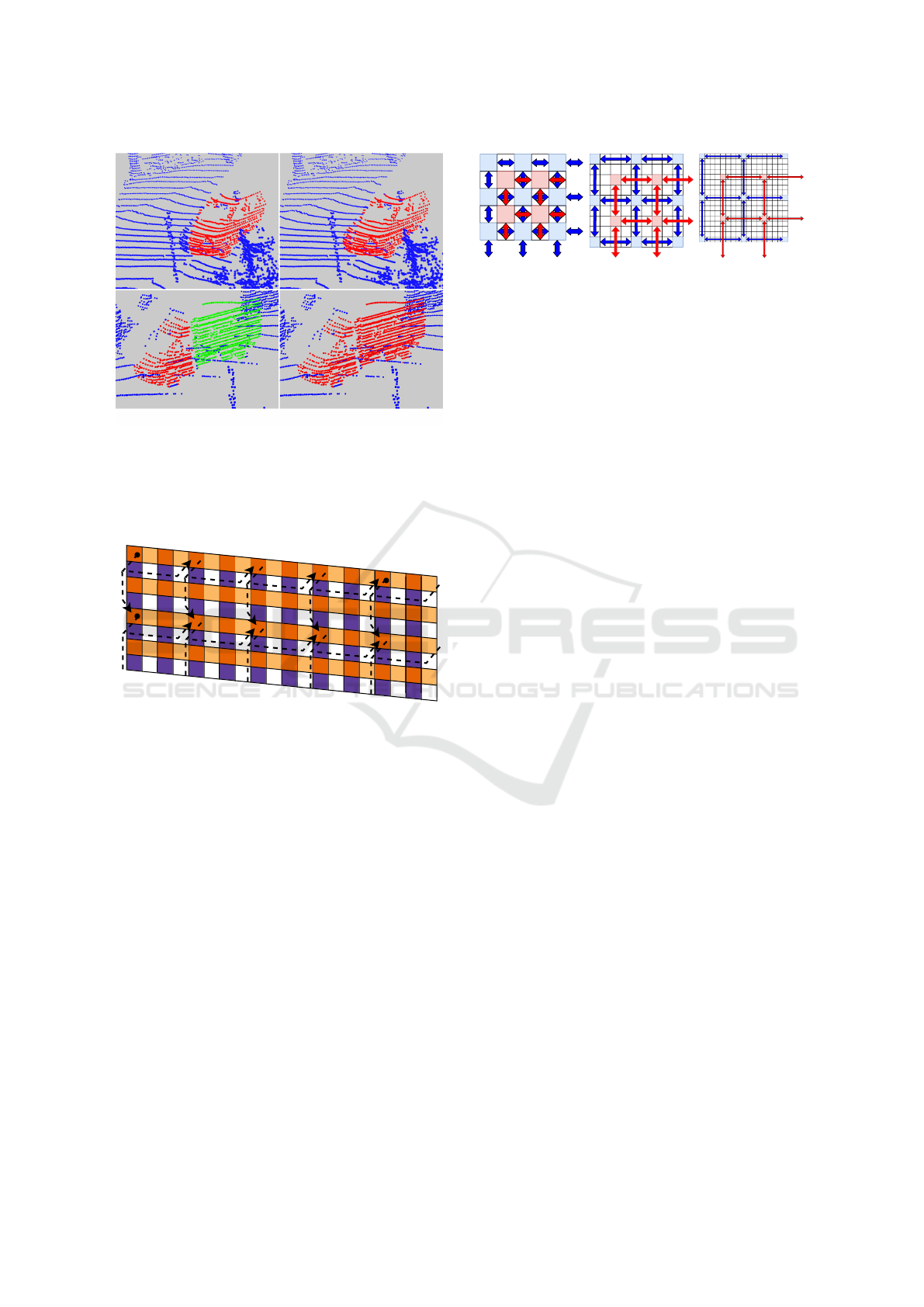
Figure 5: Left: Results using only the direct connectivity

between neighbouring Lidar points. Right: A single addi-

tional MC between every second Lidar measurement. The

proposed MCs enable a more accurate segmentation of the

car (top) and reduce the over-segmentation of partially oc-

cluded objects, as the truck in the bottom images shows.

Figure 6: Additional Map Connections (dotted lines) be-

tween non-neighbouring Lidar points on top of the di-

rect connections to neighbouring points (yellow and blue

squares).

An example of this improved segmentation can be

seen in Figure 5. In the results shown in Section 4

we have added one MC between every second mea-

surement as sketched in Figure 6, 6 MCs as shown

in Figure 7 and 14 MCs along the main diagonal of

the range image. The Maps of reduced point-sets

are smaller than the original point-set and thus re-

quire only a fraction of the computation time on top of

the directly connected clusters. The additional map-

ping of the cluster-ids of the original clusters with

the MCs, results in a slightly increased runtime as

shown in Section 4.1. The combined use of the direct

connectivity of neighbouring measurements and the

MCs enables a pseudo three-dimensional Euclidean

clustering while exploiting the fast runtime of two-

dimensional pixel connectivity. Thus, we are able to

improve the quality of the segmentation without sac-

riﬁcing our real-time ability.

Figure 7: Visualisation of the 6 Map Connection structure

for increasing the connection area with the least amount of

maps.

4 EXPERIMENTAL EVALUATION

The ﬁrst experimental evaluation measures our meth-

ods ability to run in real time at usual sensor recording

frequencies, while offering a constant processing rate

with very little ﬂuctuation independent of the scene’s

context. The second experiment is mainly concerned

with a quantitative metric of the segmentation quality.

4.1 Runtime

Following the experimental setup of (Bogoslavskyi

and Stachniss, 2016), we designed our ﬁrst exper-

iment on the provided data by Moosmann et al.

(Moosmann, 2013) to support the claim, that the pro-

posed approach can be used for online segmentation.

All listed methods have been evaluated on the same

Intel



Core

i7-6820HQ CPU @ 2.70 GHz.

Figure 8 shows the execution time of the 5 meth-

ods over the 2500 Frames dataset (Moosmann, 2013).

The proposed method runs at an average of 165 Hz

and is therefore faster than the previously fastest al-

gorithm of (Bogoslavskyi and Stachniss, 2016) at 152

Hz, while exhibiting less ﬂuctuation due to the bi-

nary image implementation when used without any

additional MCs. A box-plot of the average runtime

of (Bogoslavskyi and Stachniss, 2016) and the pro-

posed method can be seen in Figure 9, which shows

the ﬂuctuating nature of methods depending on the

scene context, as opposed to ours. As can be seen in

Figure 8, when adding MCs to the proposed methods,

the execution suffers from a slightly longer runtime,

while still running at a frequency of 26 to 105 Hz de-

pending on the number of additional MCs. This is

still between 2.6 to ten times faster than the record-

ing frequency of the used sensor. Please note that we

only used up to 14 MC in this timing. More MCs in-

crease the execution time accordingly and endanger

the real time capability of the proposed method. Im-

plementations of the Map Connection assignment in

an efﬁcient programming language like C++ might

enable the use of more MCs with less inﬂuence on

the execution time.

ICPRAM 2021 - 10th International Conference on Pattern Recognition Applications and Methods

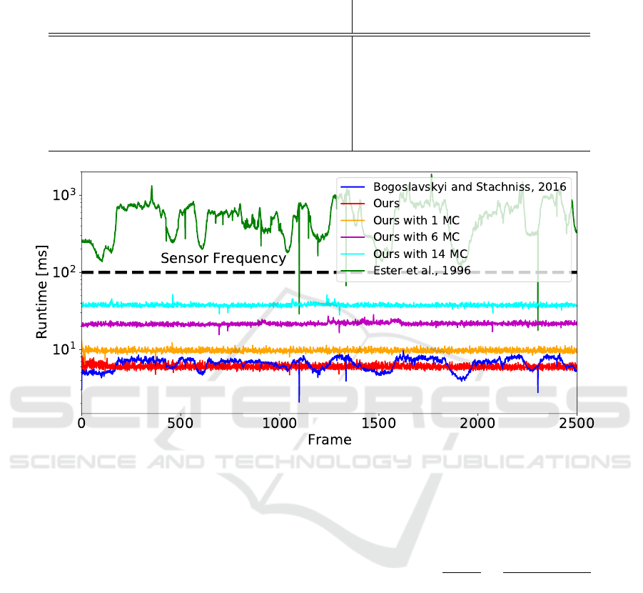
Table 1: Comparison of the segmentation quality using the Intersection over Union and the precision average for the algorithms

of (Bogoslavskyi and Stachniss, 2016), (Ester et al., 1996), and variations of the proposed method.

Method IoU

IoU

0.5

0.75

0.95

(No Ground) (Ground)

Bogoslavskyi et al. 73.93 73.93 59.31 83.75 63.52 13.18

Ours 76.20 72.31 63.73 84.30 67.51 22.03

Ours (1 MC) 77.97 73.65 66.68 85.60 70.21 27.19

Ours (6 MC) 81.14 75.48 71.92 88.25 74.99 36.05

Ours (14 MC) 84.25 76.39 74.68 89.75 77.61 40.63

DBSCAN 76.21 72.77 76.50 81.54 76.45 69.25

Figure 8: Frame-wise execution timings on a 64-beam Velodyne dataset (Moosmann, 2013). Please note the logarithmic scale

for the runtime.

4.2 Segmentation Results

For our evaluation, we use the dataset “Se-

manticKITTI” by Behley et al. (Behley et al.,

2019) as object instance segmentation ground truth.

This dataset enriches the KITTI dataset’s (Geiger

et al., 2012) odometry challenge with semantic and

instance-wise labels for every Lidar measurement.

To reduce the inﬂuence of the proposed ground

plane extraction in Section 3.1 and focus on the results

of the clustering mechanisms, we have conducted the

evaluation once without the Lidar points of the classes

road, parking, sidewalk, other-ground, lane-marking

and terrain. And a second time without any usage of

the semantic labels by applying the ground extraction

proposed in 3.1 on all methods.

For each ground truth object with at least 100 Li-

dar point measurements, we select each algorithm’s

object cluster output with the most ground truth over-

lap. Using these two lists of points, we calculate

the Intersection over Union (IoU). By averaging these

IoU values of every single instance over all 10 se-

quences, we get the averaged mean IoU

of each algo-

rithm. The IoU or Jaccard Index for a single ground-

truth instance with a single cluster is deﬁned as

J(A, B) =

|A ∩ B|

|A ∪ B|

T P

T P + FP + FN

. (5)

The connection and separation of instances solely

through the distance harbours the risk of under-

segmentation in the case of objects that are in con-

tact or are close by. For this reason, we measure

our results in the subsequent evaluation instance-wise.

If two instances are represented by only one clus-

ter, we count only the object with the higher IoU,

while the second object is marked as not found. We

compute this metric for each algorithm listed below,

over all ten sequences with Lidar instance ground

truth in the dataset. We compare the quality of

our algorithm to the currently fastest algorithm (Bo-

goslavskyi and Stachniss, 2016) as well as a very pre-

cise three-dimensional euclidean clustering algorithm

(Ester et al., 1996). We use scikit-learn’s implemen-

tation of DBSCAN (Pedregosa et al., 2011). If you

FLIC: Fast Lidar Image Clustering

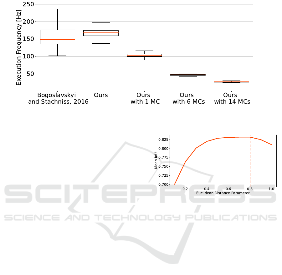
Figure 9: Averaged runtime in Hz for segmenting approximately 2,500 scans from a 64-beam Velodyne dataset (Moosmann,

2013) with our approach and up to 14 Map Connections compared to the method by Bogoslavskyi and Stachniss (Bogoslavskyi

and Stachniss, 2016).

consider the age of this algorithm, it might be sur-

prising to see that it is still used in modern cluster-

ing applications (Zhang et al., b) (Mao et al., 2020)

(Cheng et al., 2019). This long-term relevance was

also conﬁrmed by the ”Test of Time” Award from

ACM SIGKDD (SIGKDD, 2014). The algorithm was

also revisited by the original authors in a follow-up

paper (Schubert et al., 2017) fairly recently to show

the continued relevance in many clustering applica-

tions. Therefore we use the DBSCAN to compare

our pseudo three-dimensional approach to a well per-

forming three-dimensional algorithm.

We present the mean of the IoUs with the best-

performing parameters of each method. With our

threshold parameter set as 0.8m, we outperform (Bo-

goslavskyi and Stachniss, 2016) with the direct neigh-

bourhood implementation without any MCs while ex-

hibiting a faster run-time. This parameter has been set

with an additional experiment on a single log of the

dataset as can be seen in Figure 10. Other Lidar sen-

sors perform better with a higher or lower threshold

depending on the horizontal and vertical resolution of

the Lidar sensor. We recommend to evaluate the eu-

clidean distance parameter for the use of different sen-

sors. On average our method is 8% faster, while the

difference in the respectively longest execution time

of a given frame is 15%. Together with the proposed

MCs between all odd measurements, we manage to

perform higher on the average IoU than the more gen-

eral three-dimensional Euclidean distance clustering

algorithm DBSCAN (Ester et al., 1996), as shown in

Table 1.

Using 6 MCs, we surpass the performance of DB-

SCAN with a larger margin and manage to reach a

noticeably higher mean IoU. A total of 14 MCs out-

performs the three-dimensional DBSCAN algorithm

Figure 10: Parameter study of the maximum distance be-

tween two points, to be considered part of the same cluster.

The dashed line shows the maximum IoU for the evalua-

tion log. The plateau between 0.5m and 0.8m shows a very

broad and robust sweet spot for the proposed method.

on 4 of the 6 shown metrics in Table 1, with an av-

erage execution frequency of 26 Hz it still runs at 2.6

times the sensor frequency. We suspect that the re-

striction to the immediate surroundings of the mea-

surements prevents under-segmentation of separate,

close objects, but still enables the skipping of gaps

on the same object.

Without any MCs we are on average 120 times

faster. With an increasing number of additional MCs

we are 67, 25 and 14 times faster than the DBSCAN

Algorithm. Even if we drastically increase the num-

ber of MCs, our proposed method is at least 14 times

faster than the DBSCAN and remains clearly above

the sensor recording frequency.The run-time increase

does not scale logarithmically as one would expect

with additional MCs (since they apply the same func-

tion to a smaller subset of the original point cloud).

This issue might result from the mapping overhead

caused by our python implementation. We did not

re-implement the method in a different programming

language, as the computation time was still far below

ICPRAM 2021 - 10th International Conference on Pattern Recognition Applications and Methods

the sensor frequency and does not bring any further

beneﬁts to do so.

The second column of Table 1 shows, that the pro-

posed ground extraction method of Section 3.1 de-

grades the performance of all listed algorithms, ex-

cept for (Bogoslavskyi and Stachniss, 2016) as the

used metric for the ground segmentation is very sim-

ilar to the cluster separation metric used by Bo-

goslavskyi et al. A better ground separation will

lead to a much better performance for the proposed

method as the IoU values with the ground truth (GT)

ground segmentation show. Improving the ground

separation is therefore critical to improve the instance

segmentation.

For further evaluation of the instance-level per-

formance, we compute the precision similar to (Bo-

goslavskyi and Stachniss, 2016) in a more reﬁned

fashion on the GT ground removed point clouds. We

deﬁne 10 bins of point-wise overlap of the GT and

proposed clusters ranging from an IoU of 0.5 to 0.95

in steps of 0.05. We average the precision of all bins

into one single metric score (P

) which is shown in

Table 1 for each method. We additionally list the Pre-

cision for the overlap values of 0.5, 0.75 and 0.95, in

which the deﬁnition of a correctly segmented object

is deﬁned as above the denoted IoU. The precision,

which shows how many instances are matched with

an IoU of at least x is therefore deﬁned as

∑

n=0

∑

m=0

n,m

with a

n,m

(

1, if J(n, m) >= x,

0, else.

(6)

for N instances and M clusters in which each in-

stance and cluster are matched via the Jaccard Index

(IoU). Please note, that due to the deﬁnition of the

Jaccard Index only one cluster can match a ground

truth instance with an IoU > 0.5.

We show in Table 1, that we match on average

more GT instances than (Bogoslavskyi and Stachniss,

2016) and are close to the mean segmentation preci-

sion of the DBSCAN algorithm. With a higher num-

ber of MCs, we achieve better precision values for

overlap values of 0.5 and 0.75, while the DBSCAN

algorithm matches more instances with higher over-

lap values due to the full three-dimensional clustering

on all points of the dataset.

We only compare up to 14 MCs in order to not

endanger our real-time capability. However, with just

these 14 MCs, we achieve a clustering segmentation

which performs comparable to, and in some regards

better, than the full three-dimensional algorithm. The

high precision values for the lower overlap regions of

0.5 and 0.75 are particularly important in the context

of driver assistance systems, since a missed instance

can lead to dramatic outcomes, as opposed to a not

perfectly matched instance. We further proved, that

the proposed MCs improve the results of our algo-

rithm immensely and help to ﬁnd otherwise missed

objects.

Attentive readers will notice the performance of

both our method and the method by (Bogoslavskyi

and Stachniss, 2016) drop noticeably in the 0.95 IoU

bracket. We see this issue to be due to the under-

lying data. The “SemanticKITTI” dataset (Behley

et al., 2019) has a pre-applied ego-motion compensa-

tion, due to which the three-dimensional point cloud

is slightly shifted and rotated away from the origi-

nal sensor conﬁguration to compensate the movement

in the 0.1s recording time of a single frame. This

compensation has already been applied to the original

odometry dataset of Geiger et al. (Geiger et al., 2012)

to provide better Lidar odometry for static inter-frame

point cloud matching.

Our method builds on this three-dimensional point

cloud and expects an unaltered version of the Lidar

sensor to enable a one-to-one matching of the three di-

mensional points to the two-dimensional range image

representation. This can not be fully achieved with

this ego-motion compensated data and results in miss-

ing and wrongly assigned points and in turn hurts our

performance in the 0.95 IoU bracket, which requires

a precise projection. We see the same drop ampliﬁed

in the range-image based algorithm of (Bogoslavskyi

and Stachniss, 2016), while the DBSCAN algorithm

runs directly on the manipulated three-dimensional

data and does not suffer from this restriction.

5 CONCLUSION

We have presented an algorithm for real-time instance

segmentation of Lidar sensor data using raw range

images to connect points by their three-dimensional

distance. To make this approach more robust against

over-segmentation, we introduced what we call Map

Connections, which use the larger neighbouring con-

text for a more precise assignment of measured points

to an instance, especially in cases of partial occlusion.

These properties of our method facilitate the preserva-

tion of three-dimensional information in the measure-

ments when reduced to a two-dimensional represen-

tation for fast computation.

In a detailed evaluation, we have shown, that our

approach is faster than comparable state-of-the-art

methods, while being more stable in its runtime, and

more importantly, providing an overall better perfor-

FLIC: Fast Lidar Image Clustering

mance in instance segmentation. The experiments

show, that not only our accuracy in separating ob-

jects is higher than comparable fast approaches, but

we are able to match most ground truth instances

with a signiﬁcant overlap of the ground truth. This

is particularly important in the context of driver as-

sistance systems, since a missed instance is a bigger

problem than an object that was not matched with all

Lidar points. We have also illustrated, that the pro-

posed MCs improve the results of our algorithm and

help to ﬁnd otherwise missed objects. The further

use of segmented point clouds for classiﬁcation and

to remove false positives, is outside the scope of this

work. However, this application has previously been

researched by (Hahn et al., 2020) and shows promis-

ing results.

REFERENCES

AbuBaker, A., Qahwaji, R., Ipson, S., and Saleh, M. (2007).

One scan connected component labeling technique.

In 2007 IEEE International Conference on Signal

Processing and Communications, pages 1283–1286.

IEEE.

Allegretti, S., Bolelli, F., Cancilla, M., and Grana, C.

(2019). A block-based union-ﬁnd algorithm to la-

bel connected components on gpus. In International

Conference on Image Analysis and Processing, pages

271–281. Springer.

Ankerst, M., Breunig, M. M., Kriegel, H.-P., and Sander, J.

(1999). Optics: ordering points to identify the cluster-

ing structure. ACM Sigmod record, 28(2):49–60.

Behley, J., Garbade, M., Milioto, A., Quenzel, J., Behnke,

S., Stachniss, C., and Gall, J. (2019). Semantickitti:

A dataset for semantic scene understanding of lidar

sequences. In Proceedings of the IEEE International

Conference on Computer Vision, pages 9297–9307.

Bogoslavskyi, I. and Stachniss, C. (2016). Fast range

image-based segmentation of sparse 3d laser scans

for online operation. In 2016 IEEE/RSJ International

Conference on Intelligent Robots and Systems (IROS),

pages 163–169. IEEE.

Cheng, H., Li, Y., and Sester, M. (2019). Pedestrian group

detection in shared space. In 2019 IEEE Intelligent

Vehicles Symposium (IV), pages 1707–1714. IEEE.

Chu, P., Cho, S., Sim, S., Kwak, K., and Cho, K. (2017). A

fast ground segmentation method for 3d point cloud.

Journal of information processing systems, 13(3).

Comaniciu, D. and Meer, P. (2002). Mean shift: A robust

approach toward feature space analysis. IEEE Trans-

actions on pattern analysis and machine intelligence,

24(5):603–619.

Cortinhal, T., Tzelepis, G., and Aksoy, E. E. (2020). Sal-

sanext: Fast semantic segmentation of lidar point

clouds for autonomous driving. arXiv preprint

arXiv:2003.03653.

Ester, M., Kriegel, H.-P., Sander, J., Xu, X., et al. (1996).

A density-based algorithm for discovering clusters in

large spatial databases with noise. In Kdd, volume 96,

pages 226–231.

Fukunaga, K. and Hostetler, L. (1975). The estimation of

the gradient of a density function, with applications in

pattern recognition. IEEE Transactions on informa-

tion theory, 21(1):32–40.

Geiger, A., Lenz, P., and Urtasun, R. (2012). Are we ready

for autonomous driving? the kitti vision benchmark

suite. In 2012 IEEE Conference on Computer Vision

and Pattern Recognition, pages 3354–3361. IEEE.

Gerdzhev, M., Razani, R., Taghavi, E., and Liu, B. (2020).

Tornado-net: multiview total variation semantic seg-

mentation with diamond inception module. arXiv

preprint arXiv:2008.10544.

Hahn, L., Hasecke, F., and Kummert, A. (2020). Fast ob-

ject classiﬁcation and meaningful data representation

of segmented lidar instances. 23rd IEEE Interna-

tional Conference on Intelligent Transportation Sys-

tems (ITSC).

Hennequin, A., Lacassagne, L., Cabaret, L., and Meunier,

Q. (2018). A new direct connected component label-

ing and analysis algorithms for gpus. In 2018 Con-

ference on Design and Architectures for Signal and

Image Processing (DASIP), pages 76–81. IEEE.

Himmelsbach, M., Hundelshausen, F. V., and Wuensche,

H.-J. (2010). Fast segmentation of 3d point clouds for

ground vehicles. In 2010 IEEE Intelligent Vehicles

Symposium, pages 560–565. IEEE.

Hoshen, J. and Kopelman, R. (1976). Percolation and clus-

ter distribution. i. cluster multiple labeling technique

and critical concentration algorithm. Physical Review

B, 14(8):3438.

Kochanov, D., Nejadasl, F. K., and Booij, O. (2020). Kpr-

net: Improving projection-based lidar semantic seg-

mentation. arXiv preprint arXiv:2007.12668.

Korchev, D., Cheng, S., Owechko, Y., et al. (2013). On

real-time lidar data segmentation and classiﬁcation. In

Proceedings of the International Conference on Im-

age Processing, Computer Vision, and Pattern Recog-

nition (IPCV), page 1. The Steering Committee of The

World Congress in Computer Science, Computer . . . .

Lahoud, J., Ghanem, B., Pollefeys, M., and Oswald, M. R.

(2019). 3d instance segmentation via multi-task met-

ric learning. In Proceedings of the IEEE International

Conference on Computer Vision, pages 9256–9266.

Mao, J., Xu, G., Li, W., Fan, X., and Luo, J. (2020).

Pedestrian detection and recognition using lidar for

autonomous driving. In 2019 International Confer-

ence on Optical Instruments and Technology: Opti-

cal Sensors and Applications, volume 11436, page

114360R. International Society for Optics and Pho-

tonics.

Milioto, A., Behley, J., McCool, C., and Stachniss, C.

(2020). LiDAR Panoptic Segmentation for Au-

tonomous Driving.

Moosmann, F. (2013). Interlacing self-localization, mov-

ing object tracking and mapping for 3d range sensors,

volume 24. KIT Scientiﬁc Publishing.

ICPRAM 2021 - 10th International Conference on Pattern Recognition Applications and Methods

Moosmann, F., Pink, O., and Stiller, C. (2009). Segmen-

tation of 3d lidar data in non-ﬂat urban environments

using a local convexity criterion. In 2009 IEEE Intel-

ligent Vehicles Symposium, pages 215–220. IEEE.

Pedregosa, F., Varoquaux, G., Gramfort, A., Michel, V.,

Thirion, B., Grisel, O., Blondel, M., Prettenhofer,

P., Weiss, R., Dubourg, V., Vanderplas, J., Passos,

A., Cournapeau, D., Brucher, M., Perrot, M., and

Duchesnay, E. (2011). Scikit-learn: Machine learning

in Python. Journal of Machine Learning Research,

12:2825–2830.

Schubert, E., Sander, J., Ester, M., Kriegel, H. P., and Xu,

X. (2017). Dbscan revisited, revisited: why and how

you should (still) use dbscan. ACM Transactions on

Database Systems (TODS), 42(3):1–21.

SIGKDD, A. (2014). 2014 sigkdd test of time

award. https://www.kdd.org/News/view/2014-sigkdd-

test-of-time-award.

Tang, H., Liu, Z., Zhao, S., Lin, Y., Lin, J., Wang, H., and

Han, S. (2020). Searching efﬁcient 3d architectures

with sparse point-voxel convolution. arXiv preprint

arXiv:2007.16100.

Toffoli, T. and Margolus, N. (1987). Cellular automata ma-

chines: a new environment for modeling. MIT press.

Virtanen, P., Gommers, R., Oliphant, T. E., Haberland, M.,

Reddy, T., Cournapeau, D., Burovski, E., Peterson,

P., Weckesser, W., Bright, J., et al. (2020). Scipy

1.0: fundamental algorithms for scientiﬁc computing

in python. Nature methods, 17(3):261–272.

Wang, B. H., Chao, W.-L., Wang, Y., Hariharan, B., Wein-

berger, K. Q., and Campbell, M. (2019a). Ldls: 3-d

object segmentation through label diffusion from 2-

d images. IEEE Robotics and Automation Letters,

4(3):2902–2909.

Wang, Y., Yu, Y., and Liu, M. (2019b). Pointit: A fast

tracking framework based on 3d instance segmenta-

tion. arXiv preprint arXiv:1902.06379.

Yang, B., Wang, J., Clark, R., Hu, Q., Wang, S., Markham,

A., and Trigoni, N. (2019). Learning object bounding

boxes for 3d instance segmentation on point clouds. In

Advances in Neural Information Processing Systems,

pages 6740–6749.

Zermas, D., Izzat, I., and Papanikolopoulos, N. (2017). Fast

segmentation of 3d point clouds: A paradigm on li-

dar data for autonomous vehicle applications. In 2017

IEEE International Conference on Robotics and Au-

tomation (ICRA), pages 5067–5073. IEEE.

Zhang, F., Fang, J., Wah, B., and Torr, P. Deep fusionnet for

point cloud semantic segmentation.

Zhang, F., Guan, C., Fang, J., Bai, S., Yang, R., Torr, P., and

Prisacariu, V. (2020). Instance segmentation of lidar

point clouds. ICRA, 4(1).

Zhang, S., Di Wang, F. M., Qin, C., Chen, Z., and Liu, M.

Robust pedestrian tracking in crowd scenarios using

an adaptive gmm-based framework.

Zhou, H., Zhu, X., Song, X., Ma, Y., Wang, Z., Li, H., and

Lin, D. (2020). Cylinder3d: An effective 3d frame-

work for driving-scene lidar semantic segmentation.

arXiv preprint arXiv:2008.01550.

FLIC: Fast Lidar Image Clustering