
Evaluation of Knee Implant Alignment using Radon Transformation
Guillaume Pascal
1
, Andreas Møgelmose
1
and Andreas Kappel
2,3
1
Visual Analysis of People Laboratory, Aalborg University, Denmark
2
Department of Clinical Medicine, Aalborg University, Denmark
3
Interdisciplinary Orthopaedics, Aalborg University Hospital, Denmark
Keywords:
Radiograph, Total Knee Arthroplasty, Medical Image Processing.
Abstract:
In this paper we present a method for automatically computing the angles between bones and implants after
a knee replacement surgery (Total Knee Arthroplasty, TKA), along with the world’s first public dataset of
TKA radiographs, complete with ground truth angle annotations. We use the Radon transform to determine
the angles of the relevant bones and implants, and obtain 94.9% measurements within 2
◦
. This beats the
current state-of-the-art by 2.9%. The system is thus ready to be used in assisting surgeons and replacing time
consuming and observer dependent manual measurements.
1 INTRODUCTION
Knee osteoarthritis is a common cause of pain and
disability, primarily in the elderly population (Hunter
and Bierma-Zeinstra, 2019). In end-stage knee os-
teoarthritis, surgical treatment with total knee arthro-
plasty (TKA) is proven effective both in relieving pain
and restoring function (Price et al., 2018). Longevity
of the implant, pain relief, and functional outcome
following TKA surgery are all dependent on the sur-
geon’s ability to reconstruct the joint by addressing
both implant alignment and soft-tissue stability (Gro-
mov et al., 2014; Kappel et al., 2019).
Knee alignment is judged by both clinical exam-
ination and radiographs prior to the TKA operation,
and anatomical variations relevant for the procedure
are observed. During surgery, the bone cuts that will
determine TKA alignment are typically performed
with the aid of mechanical instruments, though ad-
justments are made based on both the preoperative
examination and the direct observation of bony and
other anatomical landmarks. TKA alignment is there-
fore influenced by both individual anatomical varia-
tions and by surgeon experience and preference. Be-
cause of this, variations from optimal alignment can
be observed. Routine postoperative knee radiographs
deliver feedback to the surgical team, visualizing im-
plant fixation, sizing, placement and alignment. The
Knee Society has defined standardized methods to
measure implant fixation and alignment from short
films (Meneghini et al., 2015). These measurements,
however, are time-consuming and might be observer
dependent. In our experience most institutions and
individual surgeons rely only on radiographs for non-
systematic visual feedback.
We believe that routine standardized analysis of
postoperative radiographs would deliver valuable in-
formation to both individual surgeons and institutions
and thereby further optimize the surgical outcomes.
The aim of this work was to develop a method allow-
ing fast, standardized, observer independent feedback
on coronal alignment measurement following TKA
by automation of the measurements.
In layman’s terms, the purpose of the system pre-
sented in this paper is to use a radiograph of a knee to
determine the angle between the anatomic axis of the
femur and the most distal part of the femoral implant,
as wells as the angle between the anatomic axis of the
tibia and the tibial tray. Jump ahead to fig. 14 for a
visualization of this.
2 RELATED WORK
Automated analysis of knee radiographs has been an
active research area for more than two decades. There
was a flurry of activity in the late 90s, starting with
attempts to measure the kinematics of knees using a
sequence of X-ray fluoroscopic images by comparing
a silhouette of the prosthesis to silhouettes on the im-
ages (Banks and Hodge, 1996). Similar work using
edges of implants was also presented with the use case
Pascal, G., Møgelmose, A. and Kappel, A.
Evaluation of Knee Implant Alignment using Radon Transformation.
DOI: 10.5220/0010192405870594
In Proceedings of the 16th International Joint Conference on Computer Vision, Imaging and Computer Graphics Theory and Applications (VISIGRAPP 2021) - Volume 4: VISAPP, pages
587-594
ISBN: 978-989-758-488-6
Copyright
c
2021 by SCITEPRESS – Science and Technology Publications, Lda. All rights reserved
587

of measuring wear on the polyethylene in the implant
(Fukuoka et al., 1997, 1999). Others elected to use
template matching on a library of prosthesis templates
(Hoff et al., 1996, 1998; Walker et al., 1996). Later,
a different method more capable of handling occlu-
sions was proposed (Zuffi et al., 1999). An improved
model-based method for markerless tracking of im-
plant micromotion has also been presented (Kaptein
et al., 2003).
Apart from looking at implants, a number of pa-
pers on 3D reconstruction of bones have been pre-
sented lately (Baka et al., 2011; Fotsin et al., 2019;
Kim et al., 2019; Kasten et al., 2020). For a general
overview of work in this vein, a review has also been
published (Markelj et al., 2012).
While a number of the aforementioned papers
work with knee joints and knee implants, none of
them do the post-surgical angle analysis we do in
this paper. As far as we know, only one other pa-
per tackles this problem directly (Kulkongkoon et al.,
2018). They propose a method based on a multi-
scale dual filter used to enhance bones followed by
a Canny edge detection. A linear regression model
is used to compute the bones orientation from con-
trol points while the edges of the implants are used
to compute their orientation. This method obtained
a 92% acceptance rate on a dataset of 91 X-ray im-
ages: the difference between the proposed algorithm
and the manual evaluation is two degrees or less. The
failures occured with patients who had multiple knee
replacement surgeries, and images where the two im-
plants are overlapping.
The dataset used for the test by Kulkongkoon et al.
(2018) is unfortunately not publicly available, and we
are thus unable to directly compare our performance
with theirs. Because of this, we do not only propose
a new and different angle estimation method, we also
present a public dataset of TKA radiographs available
for anybody who would like to benchmark their sys-
tem against ours.
3 DATASET
The dataset used to build and evaluate the proposed
method is composed of 137 radiographs of knees
from the AP view. Each radiograph is a grayscale
image where both implants and bones are displayed
by bright pixels, while the background and tissues are
darker. The set contains radiographs of both right and
left knees with different types of implants. Each im-
age is provided with manually labeled ground truths,
as determined by the mean measurements of two sur-
geons doing a manual evaluation of both tibial and
Figure 1: Histogram of the ground truth angle distributions
for both femoral and tibial component (alpha in black, beta
in green).
femoral angles. Having two surgeons in the pro-
cess should reduce observer bias. Histograms of the
ground truth angle distributions for both bones are
shown in fig. 1. The AAU-TKA dataset is freely
available at http://vap.aau.dk/tka.
4 RADON TRANSFORMATION
The Radon transformation is a crucial part of the pro-
posed solution, and hence we briefly describe it be-
fore going into detail about the entire system. We ap-
ply the Radon transform to highlight straight lines of
images. It is defined in equation (1) for a continu-
ous two dimensional function, or in equation (2) for a
discrete two dimensional function (Toft, 1996). The
output of the radon transformation is an image called
a sinogram. A straight line in the image can be ap-
proximated in the corresponding sinogram by a point,
whose position depends on the line position and the
orientation.
S(θ, τ) =
Z
+∞
−∞
I(x, θ x + τ)dx (1)
S(θ
k
, τ
h
) = ∆x
M−1
∑
m=0
I(x
m
, θ
k
x
m
+ τ
h
) (2)
In equation (1) S is the sinogram and I the input im-
age. θ and τ represent the slope and the offset of the
line. In equation (2) x
m
, m ∈ [0, M − 1], θ
k
and τ
k
are
the sampled x, θ and τ and ∆x is the sampling distance
of x.
5 THE PROPOSED METHOD
The method works in three stages:
VISAPP 2021 - 16th International Conference on Computer Vision Theory and Applications
588
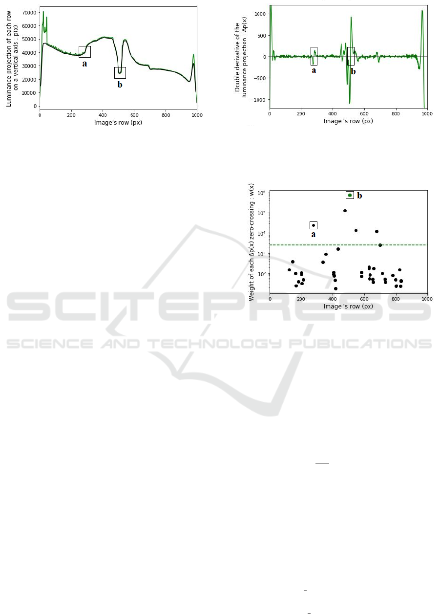
Figure 2: Luminance projection p(x) of the image on a ver-
tical axis (green). Smoothed luminance projection (black).
The shape of the implants is visible from pixels 300 to 700,
allowing to find (a) the top of the top-implant and (b) the
middle of the articulation.
Image Splitting: Divide the radiograph into three
parts: The implant, the femur, and the tibia.
Implant Orientation Estimation: Compute the ori-
entations of the two implant halves.
Bone Orientation Estimation: Compute the orien-
tation of the femur and the tibia.
In the following sections, each of these are de-
scribed in detail.
5.1 Image Splitting
Dividing the image will enable the system to focus on
each of the parts of the radiograph separately during
the following steps. The desired split looks like this:
• Implant section: The middle of the image,
bounded by a frame, will be used to find the ori-
entation of the two implants
• Femur section: The top of the image, above the
frame, will be used to compute the femur orienta-
tion
• Tibia section: The bottom of the image, below the
frame, will concern the tibia orientation. It also
contains the fibula, which is of no interest to us,
but complicates the computation slightly.
In the following paragraphs, the top left pixel is
defined as the (0,0) coordinate. The x-axis corre-
sponds to the vertical while the y-axis corresponds to
the horizontal.
The method must first find the center of the image,
defined as the middle of the articulation, and a size of
the implant section, determined by the size of the top-
implant. In short, we want to find the point (x
0
, y
0
) in
the center between the implants, and the coordinates
x
top
and x
bottom
defining the top and bottom of the im-
plant section.
Figure 3: Double derivative ∆p(x) of the luminance projec-
tion displayed on Figure (2). The markers (a) on (b) cor-
responds to the zero crossing of the corresponding markers
on Figure (2).
Figure 4: Weight of each zero crossing of the curve in Fig-
ure (3). Points above the dashed green line corresponds to
the sharpest zero-crossings: (a) is the top of the top-implant
and (b) the middle of the articulation.
To achieve this, the program calculates the lumi-
nance projection of the image on a vertical axis p(x).
Fig. 2 shows a luminance projection p(x), where we
can recognize the shape of the two implants. To ac-
curately locate the center and the top of the implant,
the double derivative ∆p(x) is computed as shown on
equation 3 below, with output displayed on fig. 3.
∆p(x) =
d
2
dx
2
"
m−1
∑
y=0
I
mb
(x, y)
#
(3)
I
mb
(x, y) is the initial n×m image successively filtered
by a median filter and a Gaussian blur. Using a me-
dian filter on the image removes the perturbation of
the clips used to close the leg after the surgery. A
Gaussian blur is also added, as the double derivative
is sensitive to noise.
A weight w(x) is determined for each zero cross-
ing in ∆p(x) as described in equation 4. This high-
lights the most sudden changes on the curve of p(x).
w(x) =
x+
τ
2
∑
i=x−
τ
2
(∆p(i))
2
∀x | ∆p(x) = 0 (4)
Evaluation of Knee Implant Alignment using Radon Transformation
589
The parameter τ represents the width of the rect-
angular function used to calculate the weight around
each zero crossing. Its value must be significantly
lower than the height of the image. Note that w(x) is
only defined for x where the double derivative ∆p(x)
is equal to zero. Fig. 4 shows the weights obtained
for each zero crossing.
The vertical position of the center of the articula-
tion x
0
(equation 5) corresponds to the zero crossing
in ∆p(x) with the highest weight because it is the most
sudden change on the representative curve of p(x), as
we can see on fig. 2.
x
0
= arg max
x
(w(x)) (5)
Following the same principle, the program is able
to find the top of the implant x
top
, as it is the zero
crossing closest to the top of the image with a weight
bigger than a certain threshold s, see eq. 6. s is defined
proportional to the maximum value of w(x).
x
top
= min({x | w(x) > s}) + ε s ∝ max(w(x)) (6)
The bottom border x
bottom
of the frame is then set
at the same distance from the center of the articulation
as the top border from the center of the articulation
(eq. 7). Even if the bottom implant is smaller than the
top implant, it remains relevant to do so since the part
of the bone close to the articulation is generally too
curved to be processed in the next steps. That is why
a margin ε is also added to expand the frame.
x
bottom
= x
0
+ (x
0
− x
top
) (7)
The final step consists of finding the horizontal po-
sition of the center of the articulation y
0
. This time,
the program computes the luminance projection q(y)
of the implant section on an horizontal axis. As shown
on eq. 8, the projection q(y) is then convolved with a
rectangular function Π(y).
y
0
= arg max
y
(q(y) ∗ Π(y)) (8)
The size of the rectangular function must be sim-
ilar to the horizontal width of the implants. Since the
implants are brighter than the background of the im-
age, the result is a concave curve with a maximum at
the middle of the articulation.
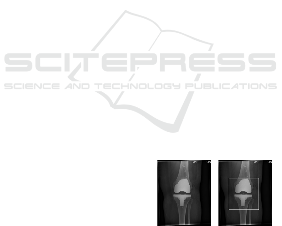
The center of the articulation can now be ex-
pressed by (x
0
, y
0
). Fig. 5 shows the final result of
the image splitting, with the center of the articulation
marked as a white dot and the white frame surrounds
the implants with a small margin.
5.2 Implant Orientation Calculation
The implant section bounded by the frame previously
defined is used when determining implant orienta-
tions. It contains the two implants. The following
method allows finding the orientation of each implant
regardless of its type and shape, based on the high
luminance difference between the implants and the
background visible at the center of the articulation.
The method is illustrated in fig. 6. The Radon
transform of the image is computed, producing a sino-
gram. In this sinogram the vertical axis corresponds
to the vertical position of a line in the image, while
the horizontal axis corresponds to the rotation a line
in the image. We can observe a dark shape in this
sinogram corresponding to all straight lines that goes
through the gap between the two implants. Focusing
on the top and bottom corner of this dark shape allows
to get the vertical position and the orientation of the
two lines tangent to the implants.
In order to improve the precision of this method,
a minimum filter is applied to the implant section to
increase the size and the contrast of the gap between
the implants, leading to a darker and bigger shape in
the sinogram, easier to segment. This operation turns
out to be particularly useful in the following cases:
• The top surface of the bottom implant is visible
on the radiograph, making its edge hardly distin-
guishable. An example is given on fig. 7. This
case appears when the patient’s leg is too flexed.
The filter smooths the image and the edge is easier
to recognize.
• The clips are disrupting the middle image. The
minimum filter simply removes these clips, also
visible on fig. 7.
• The two implants are too close to each other or
even touching as shown on Figure (8). The min-
imum filter increases the size of the gap without
changing the orientation of the implants.
(a) Initial image. (b) Obtained frame.
Figure 5: Example of final result of the image splitting.
VISAPP 2021 - 16th International Conference on Computer Vision Theory and Applications
590
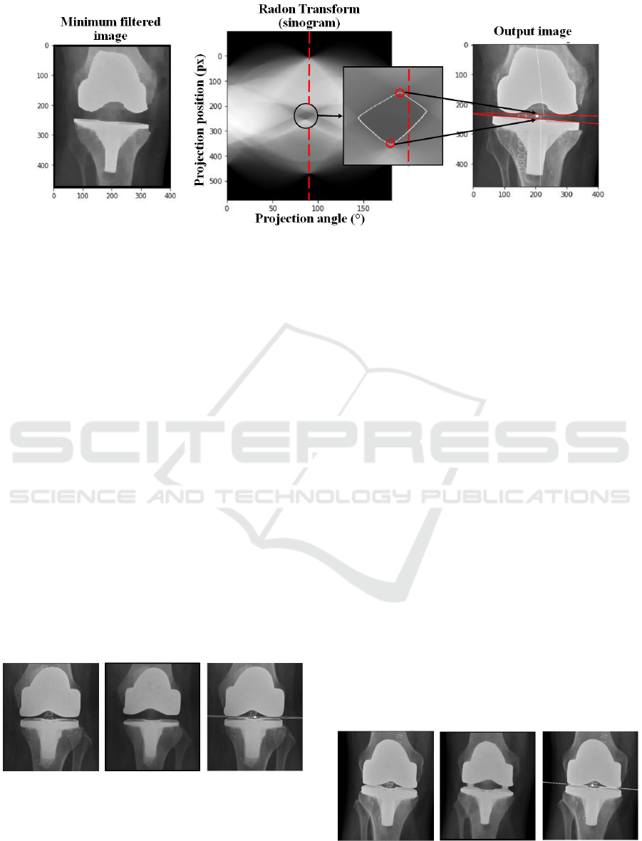
Figure 6: Method for implant orientation calculation. On the left the implant section filtered by a minimum filter is shown. The
corresponding sinogram is visible in the middle, with a zoom to its interesting part. The vertical dashed red line corresponds
to the 90
◦
projection angle. On the left the resulting lines for each implant are shown.
5.3 Bone Orientation Calculation
The orientation of a bone (femur or tibia) is calculated
as the mean of the orientation of its two edges. After
applying an edge detector, each edge is approximated
with a straight line. It is consequently important to
find a way to distinguish the correct edges from the
useless ones: the edges of the leg and the fibula inter-
fere with the edges of the femur and the tibia. Thus,
approximating the position of the interesting bones is
useful.
5.3.1 Approximate Bone Location
In order to locate the bone position, the program com-
putes the luminance projection on an horizontal axis
of both top and bottom images. As when finding the
horizontal center of the articulation, the projections
are convolved by a rectangular function of size simi-
lar to the width of the bones. The approximate center
of each bone finally corresponds to the maximum of
each resulting curve.
Figure 7: From left to right: Initial image, minimum filtered
image, resulting image. Example of radiograph processing
with flexed leg, leading to a visible top of the bottom im-
plant.
5.3.2 Edge Detection
A median filter removes the clips and the noise from
the initial image. Note that the use of a median fil-
ter changes the shape of corners, but the edges of the
bones remain unaltered. The obtained image is called
I
med
.
We find the edges as shown on eq. 9. The output
image I
edges
is equal to the difference between the 2D
maximum filtered and the 2D minimum filtered im-
age. Note that this image is not binary but shows the
magnitude of each edge.
I
edges
= max2D(I
med
) − min2D(I
med
) (9)
The kernel used is chosen according to the size
of the image, and big enough to obtain wide edges
so that even sloped bones can be considered and pro-
cessed. Sloped edges are then approximated with a
straight line.
5.3.3 Edge Orientation
The radon transform is applied on both the femur and
tibia section of I
edges
. The edges of the tibia section
is visible on fig. 10. The obtained sinogram on fig.
Figure 8: From left to right: Initial image, minimum filtered
image, resulting image. Example of radiograph processing
with top and bottom implants overlapping.
Evaluation of Knee Implant Alignment using Radon Transformation
591
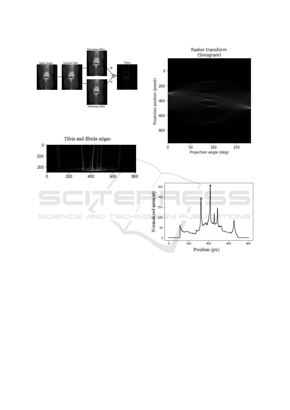
Figure 9: Edge detection method: After a median filter, the
maximum and the minimum filtered images are computed.
The image of the resulting edges corresponds to the differ-
ence between the maximum and the minimum images.
Figure 10: Edges of the tibia section. The tibia and the
fibula are visible, as well as faint lines showing the outline
of the leg.
11 contains in its center local maximums correspond-
ing to the most significant straight lines. These are
the edges of the leg, the tibia and the fibula. The pro-
gram only keeps the lines corresponding to the two
closest maximums on each side of the known approx-
imate location of the bone (see section 5.3.1). Doing
so allows to get rid of the leg and fibula perturbation,
as their maximums in the sinogram are further away.
In order to find the two closest maximums, the
maximum of each row on the sinogram is computed,
resulting in a one dimensional representative curve
(fig. 12) of the strongest line for each position, in-
dependently from their orientation. A peak detection
is then computed as follows: a peak is considered as
such if it is a local maximum considering the nearest
points. To avoid detecting a wrong one, a threshold
is set based on the intensity at the known approxi-
mate middle of the bone. Finally, the two closest
peaks from the approximate middle of the bone are
kept. The vertical and horizontal position of these two
peaks in the sinogram describes the location and the
orientation of each edge of the bone.
Figure 11: Sinogram of the tibia section edges in fig. 10.
Only the center part is kept to get the orientation of the ver-
tical lines (around a projection angle of 90
◦
) corresponding
to the bone edges.
Figure 12: Maximum intensity of each row of the sinogram,
showing the strongest edges in fig. 10 independent of the
orientation of the lines. The green dots from left to right
corresponds to the left edge of tibia (local maximum), the
approximate center of the tibia (computed previously) and
the right edge of the tibia (local maximum).
6 RESULTS
In this section we evaluate the performance of the sys-
tem. We compare the output angles with those com-
puted manually by a surgeon. However, we know that
the manual approach is observer dependent, so in a
separate test, we ask a surgeon to rate the output lines
of the system whether they follow the bones and im-
plants with sufficient accuracy.
VISAPP 2021 - 16th International Conference on Computer Vision Theory and Applications
592
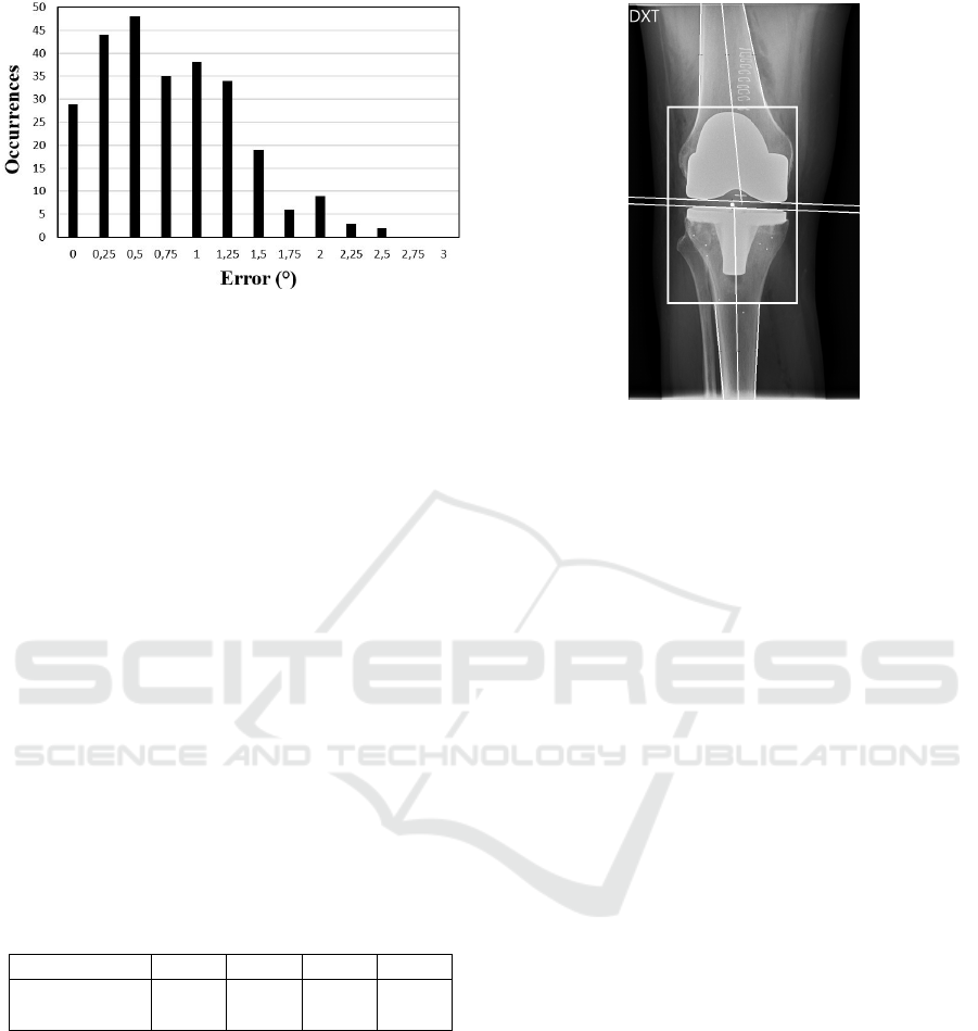
Figure 13: Error distribution on a set of 268 angles. The
error is established from the difference between manual and
automatic evaluation.
6.1 Comparison between Manual and
Computed Angles
Fig. 13 shows the error distribution of 268 computed
angles from the set of 137 images (note that 3 im-
ages were not processed by the program). The error is
defined as the absolute difference between manual re-
sults and output angles. As shown in table 1, 94.9% of
the angles are within 2
◦
from the manual evaluation.
This is generally considered acceptable, and is also
the threshold used by Kulkongkoon et al. (2018). At
94.9% we outperform their method by 2.9%, though
we are testing on a different dataset, so the results are
not directly comparable. Note that the evaluation con-
tains potential human measurement errors as well as
rounding errors on the manual measurements, since
those angles are rounded to the nearest degree. The
ground truth angles have been determined as the mean
of two evaluations made by experts in order to reduce
observer bias.
Table 1: Proportion of angles under a certain error value.
Error(
◦
) ≤ 0.5 ≤ 1.0 ≤ 1.5 ≤ 2.0
Proportion
of angles (%)
43.8 70.3 89.5 94.9
6.2 Evaluation of Output Images by
Experts
In our second test, the output images from the pro-
gram were evaluated by experts. An example is
shown on fig. 14. A check was made regarding
the correct placement of the different lines displayed:
each edge of the tibia and the femur are approximated
by a white line, as well as the resulting anatomical
axis of each bone. The orientation of each implant is
also represented by a tangent line. With a quick vi-
Figure 14: Output image of the program: The white lines
giving the orientation of the two implants are visible, as well
as the frame bounding them. Each bone edge and shaft is
also approximated by a white line.
sual control, it is simple to observe any error in the
program. The output images containing the different
lines of the process has been evaluated by experts giv-
ing 126/137 (92.0%) accepted cases.
The errors are mostly due to curved bones, wrong
approximation of bones position or images with ex-
ceptionally poor contrast.
It is worth noting that this system is intended to be
used to assist the surgeon and replace their time con-
suming manual measurements. As such it is not nec-
essarily a problem if the program fails in a few cases,
as the surgeon would be able to determine it from a
quick glance at the output image and proceed with
manual measurements if the image quality allows it.
7 CONCLUSION
In this paper, a program is presented which auto-
mates the control of radiographs following a total
knee arthroplasty. The input radiograph is split into
three parts corresponding to the femur, the implant,
and the tibia, and the orientations of each of these
are computed using the Radon transform. Along with
this paper, we publish our dataset with correspond-
ing ground truth, so other may improve on our per-
formance. When comparing with the ground truth,
94.9% of the measurements are within 2
◦
, outper-
forming the state of the art by 2.9%. The method
works with a large variety of implant shapes, and dis-
plays an output image which simple to verify by the
surgeon. The proposed method is a stable and well-
defined way to process the images, removing any ob-
Evaluation of Knee Implant Alignment using Radon Transformation
593

server bias which may be present when using manual
measurement.
REFERENCES
Baka, N., Kaptein, B. L., de Bruijne, M., van Walsum,
T., Giphart, J., Niessen, W. J., and Lelieveldt, B. P.
(2011). 2d–3d shape reconstruction of the distal fe-
mur from stereo x-ray imaging using statistical shape
models. Medical image analysis, 15(6):840–850.
Banks, S. A. and Hodge, W. A. (1996). Accurate measure-
ment of three-dimensional knee replacement kinemat-
ics using single-plane fluoroscopy. 43:638–649.
Fotsin, T. J. T., V
´
azquez, C., Cresson, T., and De Guise, J.
(2019). Shape, pose and density statistical model for
3d reconstruction of articulated structures from x-ray
images. In 2019 41st Annual International Confer-
ence of the IEEE Engineering in Medicine and Biol-
ogy Society (EMBC), pages 2748–2751. IEEE.
Fukuoka, Y., Hoshino, A., and Ishida, A. (1997). Accu-
rate 3d pose estimation method for polyethylene wear
assessment in total knee replacement. In Proceed-
ings of the 19th Annual International Conference of
the IEEE Engineering in Medicine and Biology Soci-
ety.’Magnificent Milestones and Emerging Opportuni-
ties in Medical Engineering’(Cat. No. 97CH36136),
volume 4, pages 1849–1852. IEEE.
Fukuoka, Y., Hoshino, A., and Ishida, A. (1999). A sim-
ple radiographic measurement method for polyethy-
lene wear in total knee arthroplasty. IEEE transactions
on rehabilitation engineering, 7(2):228–233.
Gromov, K., Korchi, M., Thomsen, M. G., Husted, H., and
Troelsen, A. (2014). What is the optimal alignment
of the tibial and femoral components in knee arthro-
plasty? Acta Orthopaedica, 85(5):480–487. PMID:
25036719.
Hoff, W. A., Komistek, R. D., Dennis, D. A., Gabriel, S. M.,
and Walker, S. A. (1998). Three-dimensional determi-
nation of femoral-tibial contact positions under in vivo
conditions using fluoroscopy. Clinical Biomechanics,
13(7):455–472.
Hoff, W. A., Komistek, R. D., Dennis, D. A., Walker, S.,
Northcut, E., and Spargo, K. (1996). Pose estimation
of artificial knee implants in fluoroscopy images using
a template matching technique. In Proceedings Third
IEEE Workshop on Applications of Computer Vision.
WACV’96, pages 181–186. IEEE.
Hunter, D. J. and Bierma-Zeinstra, S. (2019). Osteoarthritis.
The Lancet, 393(10182):1745 – 1759.
Kappel, A., Laursen, M., Nielsen, P. T., and Odgaard, A.
(2019). Relationship between outcome scores and
knee laxity following total knee arthroplasty: a sys-
tematic review. Acta orthopaedica, 90(1):46–52.
Kaptein, B., Valstar, E., Stoel, B., Rozing, P., and Reiber,
J. (2003). A new model-based rsa method validated
using cad models and models from reversed engineer-
ing. Journal of biomechanics, 36(6):873–882.
Kasten, Y., Doktofsky, D., and Kovler, I. (2020). End-to-
end convolutional neural network for 3d reconstruc-
tion of knee bones from bi-planar x-ray images. arXiv
preprint arXiv:2004.00871.
Kim, H., Lee, K., Lee, D., and Baek, N. (2019). 3d recon-
struction of leg bones from x-ray images using cnn-
based feature analysis. In 2019 International Confer-
ence on Information and Communication Technology
Convergence (ICTC), pages 669–672. IEEE.
Kulkongkoon, T., Cooharojananone, N., and Lipikorn, R.
(2018). Knee implant orientation estimation for x-ray
images using multiscale dual filter and linear regres-
sion model. In Meesad, P., Sodsee, S., and Unger,
H., editors, Recent Advances in Information and Com-
munication Technology 2017, pages 140–149, Cham.
Springer International Publishing.
Markelj, P., Toma
ˇ
zevi
ˇ
c, D., Likar, B., and Pernu
ˇ
s, F.
(2012). A review of 3d/2d registration methods for
image-guided interventions. Medical image analysis,
16(3):642–661.
Meneghini, R. M., Mont, M. A., Backstein, D. B.,
Bourne, R. B., Dennis, D. A., and Scuderi, G. R.
(2015). Development of a modern knee society ra-
diographic evaluation system and methodology for to-
tal knee arthroplasty. The Journal of Arthroplasty,
30(12):2311 – 2314.
Price, A. J., Alvand, A., Troelsen, A., Katz, J. N., Hooper,
G., Gray, A., Carr, A., and Beard, D. (2018). Knee
replacement. The Lancet, 392(10158):1672 – 1682.
Toft, P. (1996). The Radon Transform - Theory and Imple-
mentation. PhD thesis.
Walker, S. A., Hoff, W., Komistek, R., and Dennis, D.
(1996). ” in vivo” pose estimation of artificial knee
implants using computer vision. Biomedical sciences
instrumentation, 32:143–150.
Zuffi, S., Leardini, A., Catani, F., Fantozzi, S., and Cap-
pello, A. (1999). A model-based method for the recon-
struction of total knee replacement kinematics. IEEE
Transactions on Medical Imaging, 18(10):981–991.
VISAPP 2021 - 16th International Conference on Computer Vision Theory and Applications
594
