Multi-Mode RCPSP with Safety Margin Maximization: Models and
Algorithms
Christian Artigues
1
, Emmanuel Hebrard
1
Alain Quilliot
2
and Helene Toussaint
2
1
LAAS Laboratory, CNRS, Toulouse, France
2
LIMOS Laboratory, CNRS, Clermont-Ferrand, France
Keywords: Scheduling, Resource Constrained Project Scheduling Problem, Evacuation Process, Network Flow, Branch
and Bound, Linear Programming.
Abstract: We study here a variant of the multimode Resource Constrained Project Scheduling problem (RCPSP),
which involves continuous modes, and a notion of Safety Margin maximization. Our interest was motivated
by a work package inside the GEOSAFE H2020 project, devoted to the design of evacuation plans in face of
natural disasters, and more specifically wildfire.
1 INTRODUCTION
RCPSP: Resource Constrained Project Scheduling
Problem (see (Hartmann, 2010), Herroelen, 2005),
(Orji, 2013)) involves jobs subject to both temporal
constraints and cumulative resource constraints. In
multimode RCPSP (see (Bilseka, 2015), (Weglarz,
2011), resource requirements are flexible and the
scheduler may cut a trade-off between speed and
resource consumption. The MSM-RCPSP
(Multimode with Safety Maximization RCPSP)
model introduced is a variant of multi-mode
RCPSP: for any job j, we must choose its
evacuation rate v
j
, which determines, for any
resource e in the set Γ(j) of resources required by j,
the amount of e consumed by j. Release dates R
j
and
deadlines Δ
j
are imposed, and performance is about
safety maximization, that means the minimal
difference (safety margin), between job deadlines
and ending times.
MSM-RCPSP was motivated by the H2020
GEOSAFE European project (GeoSafe, 2018),
related to the management of wildfires. At some
time during this project, we dealt with evacuation
schedules. While in practice evacuation is managed
in an empirical way, 2-step optimization approaches
have been recently tried (see (Artigues, 2018), and
(Bayram, 2016)): the first step (pre-process)
identifies the routes that evacuees are going to
follow; the second step schedules the evacuation of
estimated late evacuees along those routes. This last
step implies priority rules and evacuation rates
imposed to evacuees and resulting models may be
cast into the MSM-RCPSP framework.
The paper is structured as follows: Section II
describes the MSM-RCPSP model. Section III
solves the fixed topology case. In Section IV we
prove that MSM-RCPSP preemptive relaxation can
be solved in polynomial time. We design in Section
V and VI both fast heuristic network flow
techniques, well-fitted to real-time management, and
an exact branch and bound algorithm. Section VII is
devoted to numerical tests.
2 MULTI-MODE RCPSP WITH
SAFETY MAXIMIZATION
MSM-RCPSP is related to a set J of jobs, subject to
release dates R
j
and deadlines Δ
j
, j ∈ J, which have
to be scheduled while maximizing what we call the
Safety Margin. That means that we want to compute
starting times T
j
and ending times T*
j
in such a way
that, for any job: R
j
≤ T
j
< T*
j
≤ Δ
j
, and that
resulting Safety Margin, defined as equal to the
quantity Inf
j
∈
J
(Δ
j
- T*
j
), is the largest possible. But
we do not know the durations of those jobs: as a
matter of fact, duration of j is determined as a
quantity P(j)/v
j
, where P(j) is some fixed coefficient
and v
j
is the speed of j, which is part of the problem
Artigues, C., Hebrard, E., Quilliot, A. and Toussaint, H.
Multi-Mode RCPSP with Safety Margin Maximization: Models and Algorithms.
DOI: 10.5220/0010190101290136
In Proceedings of the 10th International Conference on Operations Research and Enterprise Systems (ICORES 2021), pages 129-136
ISBN: 978-989-758-485-5
Copyright
c
 2021 by SCITEPRESS – Science and Technology Publications, Lda. All rights reserved
129

and which we also call evacuation rate in reference
to the Late Evacuation problem set in the context of
H2020 GEOSAFE project. The choice of those
evacuation rates is constrained in a cumulative way
by the existence of a resource set E: any job j
involves a subset J(e) ⊆ E of resources and at any
time between T
j
and T*
j
its consumption level of any
resource e ∈ E is equal to the evacuation rate v
j
,
while the amount of available resource e is bounded
by a fixed number CAP(e). Let us first link MSM-
RCPSP with evacuation problems and the
GEOSAFE H2020 Program.
2.1 Tree Late Evacuation (Tree-LEP)
We consider here a transit (evacuation) network H =
(V, E), supposed to be an oriented tree:
• Leaf subset J ⊆ V, called evacuation node set,
identifies groups of P(j) j-evacuees who must
reach the anti-root safe node SAFE while
following the arcs of related path
Γ (j). The last
j-evacuee must reach SAFE before deadline Δ
j
.
Only one arc e(j) has origin j and only one arc
has destination SAFE.
• Every arc e ∈ E is provided with time value
L(e), required for any evacuee to move along e;
L-length of
Γ (j) is denoted by Length(j). Every
arc e ∈ E is also provided with some capacity
CAP(e): no more than CAP(e) evacuees per
time unit may enter e at a given time t.
Practitioners impose that all j-evacuees move along
Γ (j) according to the same evacuation rate v
j
. This
Non Preemption Hypothesis, makes the j-evacuation
process to be determined by its starting time T
D
j
(when a first j-evacuee leaves j), its ending time T
A
j
,
(when the last j-evacuee arrives to SAFE) and its
evacuation rate v
j
, subject to (Evacuation Rate
Formula): T
A
j
= T
D
j
+ Length(j) + P(j)/v
j
.
Then the Late Evacuation Problem (LEP)
consists in the search T
D
j
, T
A
j
, v
j
, j ∈ J, consistent
with deadlines and capacities, and maximizing the
global safety margin Inf
j
(Δ
j
- T
A
j
).
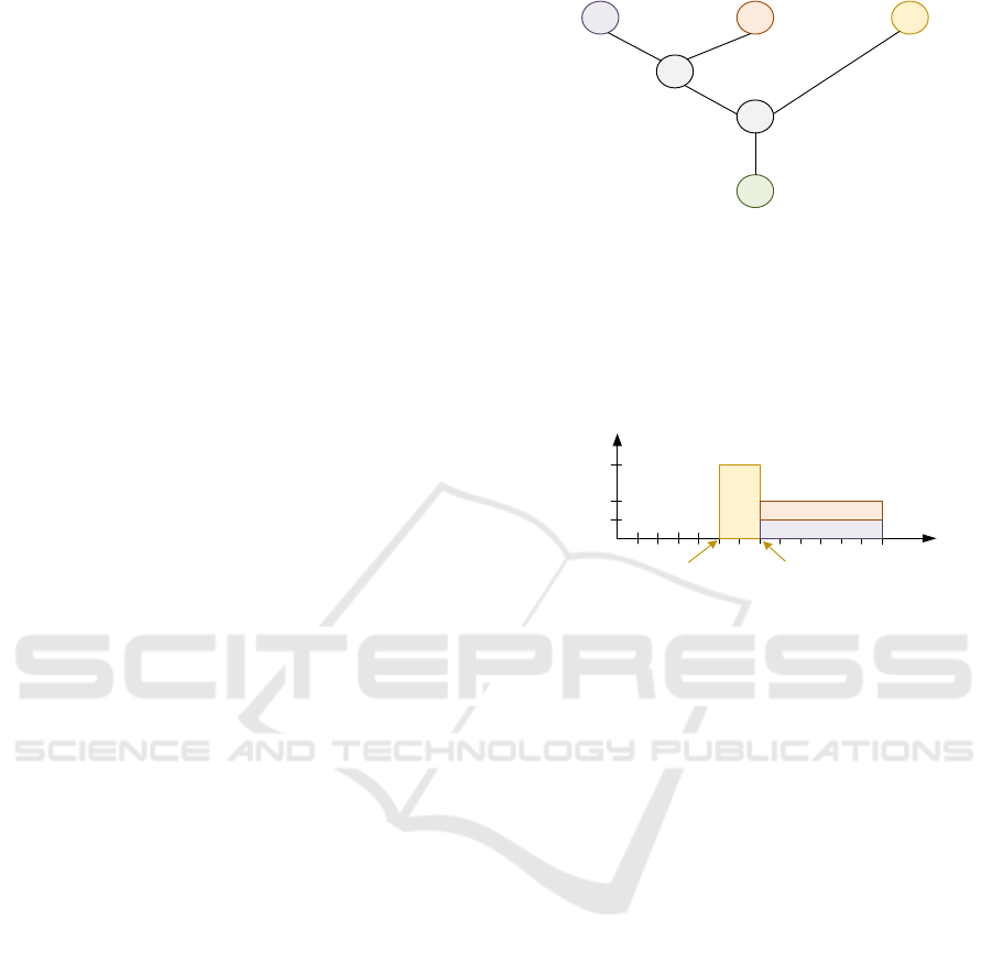
Example 1: For any arc e in Fig. 1, the first
number means the length L(e) and the second one its
capacity CAP(e). In case Δ
3
= 7; Δ
2
= Δ
1
= 13, we
make (optimal schedule) group 3 start at time zero
according to full rate v
3
= 2, and both groups 1 and 2
start at time 4, according to rates v
1
= v
2
= ½.
1 2
4
5
6
3
P(1) = 3 P(2) = 3
P(3) = 4
(1, 1) (1, 1)
(1, 1)
(1, 2)
(4, 2)
Figure 1: An Instance of Tree-LEP.
Figure 2 represents related optimal schedule
according to a Gantt diagram: The height of
rectangle j is the evacuation rate; its width is
delimited by the time when population j starts
entering node 6 and the time when it has finished.
Evacuation
rate
Time
1
1
57 13
3
2
0.5
1
2
T(3) T*(3)
Figure 2: TREE-LEP Schedule in RCPSP format.
In order to turn a Tree-LEP solution into
RCPSP format, we set, for any j in J: R
j
= Length(j)
and vmin
j
= P(j)/(Δ(j) –R
j
)). Seadline constraint
implies v
j
≥ vmin
j
; vmax
j
= CAP(e(j)). Then we
consider the process defined by the j-evacuees when
they enter into the SAFE node, and call it evacuation
job j. Its starting time is T
j
= T
D
j
+ Length(j), its
ending time is T*
j
= T
A
j
and we want to maximize
Safe-Margin = Min
j
∈
J
(Δ
j
– T*
j
). If v
j
denotes
related evacuation rate, we get the following
temporal constraints: R
j
≤ T
j
≤ T*
j
≤ Δ
j
and T*
j
= T
j
+ P(j)/v
j
. As for resource constraints, we say that 2
jobs j
1
, j
2
, overlap iff interval [T
j1
, T*
j1
] ∩ [T
j2
, T*
j2
]
is neither empty nor reduced to one point. Then
resource constraints tells that for any arc e in A and
for any Overlap clique J
0
⊆ J(e) ={j such that e ∈
Γ(j)}, we should have: Σ
j
∈
J0
∩
J(e)
v
j
≤ CAP(e). In
case J
0
= e(j), this yields v
j
≤ vmax
j
.
2.2 The MSM-RCPSP Model
According to 2.1, MSM-RCPSP Inputs are: The
job set J and the resource set E; for any j ∈ J,
Population coefficient P(j), Release date R
j
,
Deadline Δ
j
, maximal evacuation rate vmax
j
and set
subset Γ(j) ⊆ E of resources used by j; for any e ∈ E,
the Capacity CAP(e) = and the subset J(e) ⊆ E of
ICORES 2021 - 10th International Conference on Operations Research and Enterprise Systems
130

jobs j which use e. Then MSM-RCPSP model,
conjectured to be NP-Hard, comes as follows:
MSM-RCPSP Model: Compute Rational Vectors
T = (T
j
, j = 1..N), T* = (T*
j
, j = 1..N), v =
(v
j
, j = 1..N) ≥ 0, and {0, 1, -1}-valued
vector Π = (Π
j1,j2
, j
1
, j
2
= 1..N) with
Semantics : Π
j1,j2
= 1 ~ j
1
<< j
2
; Π
j1,j2
= -1 ~
j
2
<< j
1
; Π
j1,j2
= 0 ~ j
1
Overlap j
2
, such that:
• Structural Constraints: For any j
1
, j
2
,
Π
j1,j2
= - Π
j2,j1
.
• Temporal Constraints:
o For any j: R
j
≤ T
j
≤ T*
j
≤ Δ
j
and
T*
j
= T
j
+ P(j)/v
j
; (E1)
o For any pair j
1
, j
2,
the following implication
holds: Π
j1,j2
= 1 -> T
j2
≥ T*
j
; (E1*)
• Resource Constraints:
o For any j : vmin
j
= P(j)/(Δ(j) –R
j
))
≤ v
j
≤ vmax
j
;
o For any arc e, (E2) implication holds: (E2)
(J
0
⊆ J is such that for any pair j
1
, j
2
in J
0
,
Π
j1,j2
= 0) -> Σ
j
∈
J0
∩
J(e)
v
j
≤ CAP(e);
• Maximize : Safe-Margin = Inf
j
(Δ(j) – T*
j
)}
This model fits with industrial contexts, where jobs j
involving continuous flows of items are applied a
sequence Γ(j) = {e
j
1
, e
j
2
, .., e
j
n(j)
} of operations, and
pipe-lined through some set of machines.
3 FIXING THE TOPOLOGY
It will happen in next sections that we are provided
with some topological vector Π. So we denote by
MSM-RCPSP(Π) resulting MSM-RCPSP model.
MSM-RCPSP(Π) model is convex. In order to
linearize MSM-RCPSP(Π), we replace, for any j,
T*
j
by T
j
+ P(j)/v
j
, and reformulate (E1) as:
o For any j, and any w ∈ [vmin
j
, vmax
j
]: (Δ
j
-
RMin - T
j
) ≥ (- v
j
+ w).P(j)/w
2
+ P(j)/w.
This constraints tells us that for any w the 2D-point
(v
j
, (Δ
j
- T
j
- RMin)) must be located above the
tangent line in (w, P(j)/w) to the hyperbolic curve
whose equation is x -> P(j)/x. We proceed the same
way with E1* and get the following linear
formulation LINEAR-MSM-RCPSP(Π):
LINEAR-MSM-RCPSP(Π): {Compute T = (T
j
, j =
1..N), v = (v
j
, j = 1..N) ≥ 0 and RMin ≥ 0, s.t:
• Temporal constraints:
o For any j : R
j
≤ T
j
;
o For any j and any w ∈ [vmin
j
, vmax
j
]: (E1)
(Δ
j
– Rmin - T
j
) ≥ (- v
j
+ w).P(j)/w
2
+ P(j)/w;
o For any j
1
, j
2
s.t Π
j1,j2
= 1, any w ∈ [vmin
j1
,
vmax
j1
]: (E1*)
T
j2
- T
j1
≥ (- v
j1
+ w).P(j
1
)/w
2
+ P(j
1
)/w;
• Capacity Constraints:
o For any j : vmin
j
≤ v
j
≤ vmax
j
;
o For any e, any subset J
0
⊆ J s.t for any j
1
, j
2
in
J
0
, Π
j1,j2
= 0: Σ
j
∈
J0
∩
J(e)
v
j
≤ CAP(e); (E2)
• Maximize: Safe-Margin = RMin}.
We apply a cutting plane process to (E1, E1*):
Linear-MSM-RCPSP-Cut(Π):
Initialize a set W of constraints (E1, E1*) and
condider related restriction LINEAR-MSM-
RCPSP(Π, W); Not Stop ;
While Not Stop do
Solve LINEAR-MSM-RCPSP(Π, W);
Search for j
0
(j
1
, j
2
) and w
0
such that (E1,
E1*) do not hold;
If Fail(Search) then Stop
Else Insert (E1, E1*) related to j
0
, w
0
into W.
4 PREEMPTIVE MSM-RCPSP
Preemptive MSM-RCPSP means that jobs may stop
at some time and start again a little later.
Preemption allows any job j to be split into k(j) sub-
processes j
1
,.., j
k(j)
, each with starting time t
j,k
, ending
time t*
j,k
, and evacuation rate v
j,k
. We denote by P-
MSM-RCPSP the resulting problem. Figure 3
below shows an example of preemptive schedule
related to example 1.
Figure 3: P-MSM-RCPSP Schedule.
Let us now suppose that we are provided with
some safety margin λ ≥ 0 which we want to ensure.
Then we set S = {R
j
, (Δ
j
– λ), j ∈ J} and label its
elements {t
1
,.., t
2N
}, in such a way that t
1
≤ t
2
≤… ≤
t
2N
. For any k = 1,…,2N-1, we set δ
k
= t
k+1
– t
k
. This
leads to the following rational PL Preemptive(λ):
Preemptive(λ) Linear Program: Compute
rational vector w = (w
j,k
, j ∈ J, k = 1..2N-1) ≥ 0,
Multi-Mode RCPSP with Safety Margin Maximization: Models and Algorithms
131

whose semantics is that w
j,k
is the evacuation rate for
j between t
k
and t
k+1
, and which satisfies the
• For any j, k, w
j,k
≤vmax
j
;
• For any j, Σ
k
δ
k
.w
j,k
= P(j);
• For any arc e, any k: Σ
j
∈
J(e)
w
j,k
≤ CAP(e);
• For any j and any k such that t
k+1
≤ R
j
, w
j,k
= 0 ;
• For any j, k such that t
k
≥ (Δ
j
– λ): w
j,k
= 0}.
Lemma 1: Preemptive(
λ ) identifies a
preemptive schedule which is consistent with safety
margin
λ , in case such a schedule exists.
Proof: If a preemptive schedule exists, consistent
with safety margin λ, release dates R
j
, deadlines Δ
j
, j
∈ J, and capacities CAP(e), e ∈ A, then it can be
chosen in such a way that for any job j and any k,
related evacuation rate of j is constant between t
k
and t
k+1
. Then we get above linear program. 
We solve P-MSM-RCPSP by applying the
following binary process Optimal-P-MSM-RCPSP,
which computes optimal safety margin λ-Val by
making λ iteratively evolve between a non feasible
value λ
1
and a feasible one λ
0
:
Optimal-P-MSM-RCPSP(Threshold):
λ
0
<- 0 ; λ
1
<- Inf
j
[Δ(j) – (R
j
+ P(j)/vmax
j
)]; w-Sol
<- Nil ;
λ− Val <- - ∞ ; Solve Preemptive(λ
1
);
If Success(Solve) then
λ− Val <- λ
1
; w-Sol <- related
vector w
Else
Solve Preemptive(λ
0
);
If Success(Solve) then
λ− Val <- λ
0
; w-Sol <- related vector w ;
Counter <- 0;
While Counter ≤ Threshold do
λ <- (λ
1
+λ
0
)/2 ; Solve Preemptive(λ);
If Success(Solve) then λ
0
<- λ ; λ− Val <-
λ
0
; w-Sol <- related w Else λ
1
<- λ ;
Optimal-P-MSM-RCPSP <- (
λ− Val, w-
Sol);
Else Optimal-P-MSM-RCPSP <- Fail;
Theorem 1: Optimal-P-MSM-RCPSP solves the P-
MSM-RCPSP Problem in Polynomial Time.
Proof: Optimality comes in straightforward way
from the very meaning of linear program
Preemptive(λ). As for complexity, we set Threshold
= Log
2
(Sup
j
Maximal binary encoding size of Δ
j
and R
j
+ 1) and derive Time-Polynomiality from
time polynomiality of LP.€
Sterilization: We may try to turn w into a non
preemptive schedule through 2 approaches:
• Sterilization1: Smoothing w while keeping safety
margin λ as in Figure 4 below:
Evacuation
Rate (w
j
)
Time
U
1
U
3
U
4
U
5
U
6
U
9
v
j
kmin(j) = 2
kmax(j) = 7
U
2
U
8
T
j
= U
2
T*
j
= U
8
U
7
w
j
,
3
Evacuation
rate
Time
T
j
= U
2
T*
j
= U
8
v
j
Preemptive solution for job j
Non Preemptive solution for
job j after Sterilization 1
Figure 4: Sterilization1 Scheme.
• Sterilization2: Deriving from w a topological
vector Π, and solving MSM-RCPSP(Π).
5 A FLOW BASED HEURISTIC
This section is devoted to the description of a
network flow based heuristic, which implements
insertion mechanisms as in (Quilliot, 2012), and
computes an efficient feasible MSM-RCPSP
solution. We consider resources e as flow units, that
jobs j share or transmit: If we represent every job as
a rectangle whose length is the duration T*
j
– T
j
and
height is the evacuation rate v
j
, then, if j
1
precedes
j
2
, and if not jobs j is located between j
1
and j
2
on the
e-diagram, then we see (fig. 2 and 6) that part of
evacuation rate v
j1
related to resource e is
transmitted to j
2
. In order to formalize this, we build
an auxiliary network G in which the vertex set is J ∪
{s, p}, where s and p are two fictitious jobs source
and sink, whose arcs are all arcs (i, j), i, j ∈ J,
augmented with all arcs (s, j) and all arcs (j, p). Then
we consider that the backbone of a schedule is a
flow vector w = (w
e
j1,j2
, j
1
, j
2
∈ J(e) ∪ {s, p}) ≥ 0,
which represents, for all resources e, the way jobs
share resource e. Clearly, this vector w must satisfy
standard flow conservation laws:
• For any e: Σ
j
∈
J
w
e
s,j
= Σ
j
∈
J
w
e
j,p
= w
e
p,s
= CAP(e);
• For any resource e of E and any job j
0
∈ J(e), Σ
j
∈
J
∪
{p}
w
e
j0,j
= Σ
j
∈
J
∪
{s}
w
e
j,j0
= v
j0
.
Besides, if we introduce starting times T
j
and
ending times T*
j
as in II, then, for any j
1
, j
2
, the
following implication is true: Σ
e
w
e
j1,j2
≠ 0 -> T
j2
≥
T*
j1
. This logical constraint means that if job j
1
provides j
2
with some part of resource e, then j
1
should be achieved before j
2
starts. Clearly, we must
keep on with the other standard constraints:
• For any j: R
j
≤ T
j
≤ T*
j
≤ Δ
j
; v
j
≤ vmax
j
; T*
j
= T
j
+ P(j)/v
j
; T
s
= T*
s
= 0.
• Maximize Min
j
(Δ
j
– T*
j
).
ICORES 2021 - 10th International Conference on Operations Research and Enterprise Systems
132

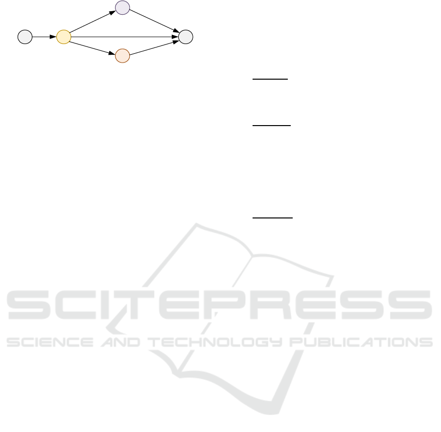
s
1
2
3 p
2
0.5
1
0.5
0.5 0.5
Figure 5: Example 2, with Δ
3
= 7, Δ
1
= Δ
2
= 13.
5.1 An Adaptative Insertion Heuristic
We deal with MSM-RCPSP-Flow through an
insertion algorithm which manages two antagonistic
trends: when handling job j and trying to insert it
into a current partial schedule (T, T*, v), we first
compute T
j
and next assign v
j
a value. But if we
choose a high value v
j
in order to make j finish fast,
then we may block the access to the most critical
resources of
Γ (j). In order to find a compromise we
control an adaptative safety margin λ through binary
search and a related adaptative priority list σ, which
drives the insertion process for a given λ. For a
given value of λ, and a current list σ, the procedure
Insert-MSM-RCPSP (λ, σ) scans the jobs j
0
in σ,
and try to compute T
j0
and v
j0
in such a way that
MSM-RCPSP-Flow constraints are satisfied for all
jobs j before or equal to j
0
according to σ, and that
v
j0
is minimal. In case of success, then λ is
increased, else Insert- MSM-RCPSP(λ, σ) yields a
set of pairs j
1
, j
2
, asked to become such that j
2
σ j
1
(Instruction Update(σ) below).
MSM-RCPSP-Flow(Precision:Number)
Algorithmic Scheme:
Step 1: Start from a non feasible margin λ-max,
a feasible one λ-min, a related Current-Schedule;
Initialize priority list σ: priority given to jobs j
with small P(j) and expected safety;
While (λ-max - λ-min) ≥ Precision do
λ <- (λ-min + λ-max )/2; Insert-MSM (λ, σ)
If Success then set λ-min to λ and Update
Current-Schedule
Else Update(σ); Retrieve topology Π from
Current-Schedule;
Step2: Solve resulting P-MSM-RCPSP(Π).
5.2 Insert-MSM Procedure
This procedure works while scanning current
priority list σ and assigning T
j
and v
j
values as far as
jobs j come. That means that at any time during the
process, we are considering some job j
0
, while all
jobs j such that j σ j
0
have been scheduled: for any j
∈ J ∪ {s} such that j
σ j
0
, we are provided with
values T
j
, T*
j
, v
j
, as well as with values Φ(e, j) which
represents the amount (evacuation rate) of e-
resource that j is able to transmit to j
0
, according to
flow vector w
e
of the MSM-RCPSP-Flow model.
Then we proceed in 3 steps:
- 1st Step: Scan
Γ (j
0
) according to decreasing
Φ(e, j
0
) values, and for any e in Γ (j
0
), provide j
0
with an amount of resource e in such a way
resulting T*
j0
does not exceed Δ
j0
- λ.
- 2nd Step: In case of success of previous first
step, we become provided with an evacuation
rate v
j0
and, for any resource e ≠ e
0
in Γ (i
0
) with
an evacuation rate value v-aux
e
which may be
less than v
i0
; So the second step makes increase
the values w
e
j,i0
for any e ≠ e
0
, j ∈ J(e), in order
to make j
0
run according to the same
evacuation rate for all arcs e of
Γ (j
0
).
- 3rd Step: In case of success of previous
second step, last step is a clustering step, which
aims at making decrease the number of
resources provided with non null w
e
j,i0
values,
and works by shifting, as far as possible, values
w
e
j,i0
which involve, for a given j, only one
resource e, to another job j’ such that j’ ∈ J(e),
w
e
j’,i0
≠ 0 and Π( e, j’) ≥ w
e
j,i0
+ w
e
j’,i0
.
Example 2: Suppose that we face here the
following situation: σ = s,…, j
1
, …, j
2
, ….j
3
, …., j
0
;
Γ (x
0
) = {e
1
, e
2
}; CAP(e
1
) = 20, CAP(e
2
) = 25; Δ
j0
=
21; P(j
0
) = 5; R
j0
= 10; j
1
∈ J(e
1
) ∩ J(e
2
); j
1
∈ J(e
1
);
j
3
∈ J(e
2
); P(j
1
)/v
1
= 6; P(j
2
)/v
2
= 3; P(j
3
)/v
3
= 4.
 Then we get:
Step1 -> w
e1
s,j0,
= 2; w
e2
s,j0
= 3; w
e1
j1,j0
= 8; v
j0
=
10; Success;
Step2 -> w
e2
j2,j0
= 7; Success; Step3 -> w
e1
j1,j0
=
0; w
e1
j2,j0
= 8; T
j0
= 21.
6 AN EXACT ALGORITHM
This Branch&Bound algorithm relies on sections IV
and V: Optimistic estimation (upper bound) derives
from IV, and an initial feasible solution is computed
according to V. We must specify:
- The nodes of related search tree and the way
optimistic estimation is adapted to those nodes;
- The Branching Strategy and the global Tree
Search process.
The nodes of the Search Tree: Such a node s
will be defined by a Release vector A = (A
j
, j ∈ J) ≥
R = (R
j
= j ∈ J), a Deadline vector B = (B
j
, j ∈ J) ≤ Δ
Multi-Mode RCPSP with Safety Margin Maximization: Models and Algorithms
133

and 2 partially defined Medium vectors U = (U
j
, j ∈
J(s)), U* = (U*
j
, j ∈ J(s) such that :
o J(s) denotes the set of jobs j such that U
j
and
U*
j
are defined;
o If j ∈ J(s), then A
j
≤ U
j
< U*
j
≤ B
j
;
For a given job j, the meaning of U
j
and U*
j
, j ∈ J(s)
is that w
j
= w
j
(t) must be constant on [U
j
, U*
j
] and
such that, for any t’ outside [U
j
, U*
j
], t inside [U
j
,
U*
j
], w
j
(t) ≥ v
j
(t’). Then Branching from s. Given a
job j and 2 values α and β such that A
j
< α < β, node
s gives rise to 3 sons:
• First son: A
j
is replaced by α;
• Second son: B
j
is replaced by β;
• Third son: U
j
is replaced by α and U*
j
by β:
we must have: α < U
j
<U*
j
< β.
The 3-uple (j, α, β) defines the Branching
Signature. Once created, node s is applied an
optimistic estimation procedure, and next, in case
Sterilization does not work, stored into a Breadth-
First Search list together with resulting value λ-Val
and related Branching Signature Sign = (j
0
, α
0
, β
0
).
Optimistic Estimation and Sterilization
Procedures: They derive from Section IV: we solve
P-MSM-RCPSP augmented with additional
constraints related to node s. More precisely:
• For any j, we set B*
j
= Inf (B
j
, Δ
j
– λ) and S =
{A
j
, B*
j
, j ∈ J} ∪ {U
j
, U*
j
, j ∈ J(s)}. We order S
= {t
1
,…, t
k
,…t
K
} through increasing values t
1
<t
2
< … < t
K
and set, for any k = 1.. K-1: δ
k
= t
k+1
- t
k
• We build 4 vectors k1, k2, k3, k4, with
indexation on J, and whose meaning is:
- k1
j
means the value k such that A
j
= t
k
;
- k2
j
means the value k such that B*
j
= t
k
;
- k3
j
means the value k such that U
j
= t
k
; (* If
U
j
is undefined, then k3
j
= 0*)
- k4
j
means the value k such that U*
j
= t
k
; (*If
U
j
is undefined, then k4
j
= 0*)
According to this, we adapt the program
Preemptive(λ) to node s by setting:
Preemptive
s
(λ): {Compute w = w
j,k
, j ∈ J, k =
1..K-1} such that;
• For any e and any k, Σ
j
∈
J(e)
w
j,k
≤ CAP(e)
• For any j, Σ
k
δ
k
. w
j,k
= P(j)
• For any j, any k ≤ k1(j) – 1, w
,k
= 0 ;
• For any j, any k ≥ k2(j), w
j,k
= 0 ;
• For any j, any k ≥ k3(j), w
,k+1
≤ w
,k
;
• For any j, any k ≤ k4(j)-2, w
j,k+1
≥ w
j,k
.
We try to turn a solution of Preemptive
s
(λ) into
a MSM-RCPSP Solution through procedures
Sterilizationx , x = 1, 2 of IV, and adapt Optimal-P-
MSM-RCPSP into a procedure UB in order to make
it compute, for a given node s = (A, B, U, U*),
related optimistic estimation λ-Val = UB(s).
Branching Strategy: Let us suppose that we just
computed λ-Val = UB(s), got a preemptive solution
w, which we could not turn into a non preemptive
solution with better Safety Margin than our current
best feasible value. Then, for any job j, we scan the
index set 1..K, and compute a word Σ
j
= {Σ
j
1
,.., Σ
j
K
}
representative of the resource profile induced by j:
o If ε = 1 then w
j,k
> w
j,k-1
;
o If ε = -1 then w
j,k
< w
j,k-1
;
o If ε = 0 then w
j,k-1
= w
j,k
and h =0.
This word Σ
j
enables us to identify:
- 1
st
Configuration: A hole (see Fig. 6) with some
depth and width and a weight = depth.width;
- 2
sd
Configuration: No hole but a left stair or a
right stair with once again a depth, a width and a
weight.
Evacuation
Rate (w
j
)
Time
α
β
Figure 6: Hole (1st Configuration) Branching.
So our Branching Strategy comes as follows: In
case Configuration 1, then we compute branching
signature Sign as some related Sg with largest
weight = depth.width. In case it does not exist, then
we look for Sg related to configuration 2 with the
highest weight value.
Resulting Branch and Bound Algorithm B&B-
MSM-RCPSP: B&B- MSM-RCPSP is implemented
as follows, according to a BFS (Breadth First
Search) strategy. In case of interruption, we get a
lower bound BInf and an upper bound BSup.
7 NUMERICAL EXPERIMENTS
Technical Context: Algorithms are implemented in
C++, gcc 7.3. Linear models are solved with Cplex
12.8. Hardware involves Processors Intel(R)
ICORES 2021 - 10th International Conference on Operations Research and Enterprise Systems
134

Xeon(R) CPU E7-8890 v3 @ 2.50 GHz, run by
Linux.
Instance Generation: Instances come from the
GEOSAFE project (see (
Artigues, 2018)). They are
clustered into 10 instance groups dense_x,
medium_x, sparse_x, where x is the number of jobs,
and dense, medium and sparse are related to the
mean degree of the nodes in related tree.
Table 1: Characteristics of the Instances.
Instances Nodes Cap-Relax Congest
dense_10 19.80 155.06 1.69
dense_15 29.10 160.08 1.78
dense_20 38.60 164.88 1.84
medium_10 19.70 152.83 1.71
medium_15 29.10 159.39 1.80
medium_20 38.20 160.69 1.86
medium_25 46.80 169.91 1.91
sparse_10 19.50 146.17 1.75
sparse_15 28.80 153.92 1.87
sparse_20 38.30 157.78 1.87
sparse_25 47.60 154.73 1.89
For any 10 instances group, above Table 1
provides us with: the mean number Nodes of nodes,
the minimal duration Cap-Relax of the evacuation
process in case capacity constraints are relaxed and
the mean (for all nodes x) ratio Congest, between the
sum of capacities of the in-arcs and the capacity of
the out-arc related to x.
7.1 Evaluating Optimal-P-MSM-
RCPSP and MSM-RCPSP-Flow
We focus here on the ability of Optimal-P- MSM-
RCPSP and MSM-RCPSP-Flow to provide us with
a good MSM-RCPSP Lower/Upper approximation
window. Table 2 provides, for every instance group:
• Opt-P-MSM: Optimal safety margin (Optimal-
P-MSM-RCPSP); Opt-P-CPU: Related CPU
time;
• # fails: the number of instances for which
MSM-RCPSP-Flow yields a fail result;
• MSM-Flow: Safety margin computed by MSM-
RCPSP-Flow; Flow-CPU: Related CPU Time;
• Preempt-Gap: the gap between MSM-Flow and
the Opt-P-MSM.
Table 2: Behavior of MSM-RCPSP-Flow.
Instances Opt-P-MSM Opt-P-CPU
dense_10 106.25 0.05
dense_15 68.3 0.08
dense_20 39.29 0.11
medium_10 92.59 0.04
medium_15 65.35 0.08
medium_20 54.85 0.11
medium_25 49.55 0.32
sparse_10 113.78 0.04
sparse_15 78.33 0.06
sparse_20 64.45 0.11
sparse_25 21.69 0.45
Table 3: Bis: Behavior of MSM-RCPSP-Flow.
Instances
MSM-
Flow
Preempt-
Gap
Flow-
CPU
#
fails
dense_10 97.09 9.23 2.01 0
dense_15 58.02 20.96 2.31 0
dense_20 34.75 20.03 2.97 2
medium_10 88.76 4.21 2.06 0
medium_15 52.87 18.24 2.82 0
medium_20 43.75 20.85 3.53 2
medium_25 36.78 26.87 1.96 1
sparse_10 110.38 3.65 1.88 0
sparse_15 75.77 3.24 2.75 0
sparse_20 48.70 28.50 3.94 0
sparse_25 32.67 * 1.18 4
Comment: Optimal-P-MSM-RCPSP and MSM-
RCPSP-Flow provide us with respectively efficient
optimistic and realistic approximations.
7.2 Evaluating B&B-MSM-RCPSP
We focus here on the filtering process and the
number of nodes of the search tree which are visited
during the process. We compute (Table 3):
• The value Opt-P-MSM as in Table 2;
• The lower (feasible) bound B&B- MSM-Inf
provided by B&B-MSM-RCPSP; The lower
bound B&B-MSM-Sup provided by B&B-
MSM-RCPSP; Related CPU time B&B- CPU;
• The number Nodes of nodes of the search tree
which were visited during the process.
Multi-Mode RCPSP with Safety Margin Maximization: Models and Algorithms
135

Table 4: Behavior of B&B- MSM-RCPSP.
Instances
Opt-P-
MSM
B&B-
MSM- Inf
B&B-
MSM-Sup
dense_10 106.25 105.75 105.76
dense_15 68.30 66.65 67.49
dense_20 39.29 38.86 39.29
medium_10 92.58 91.87 91.87
medium_15 65.35 63.42 64.48
medium_20 54.85 49.82 54.57
medium_25 51.60 49.19 51.60
sparse_10 113.78 113.75 113.78
sparse_15 78.33 78.33 78.33
sparse_20 64.45 59.21 64.38
sparse_25 34.34 32.49 34.34
Table 5: Bis: Behavior of B&B-MSM-RCPSP.
Instances Nodes B&B-CPU
dense_10 12077.80 361.14
dense_15 27148.80 1090.40
dense_20 11338.90 720.85
medium_10 4253.30 105.51
medium_15 28850.20 1440.62
medium_20 27254.90 1800.03
medium_25 10839.00 1081.33
sparse_10 57425.50 604.36
sparse_15 10668.30 360.32
sparse_20 15164.50 1440.08
sparse_25 17054.10 1800.28
Comment: B&B-MSM-Inf is always very close to
optimistic estimation Opt-P-MSM, and Optimal-P-
MSM-RCPSP provides us with a very good
approximation of optimality. Still, it is difficult to
make this optimistic estimation decrease.
8 CONCLUSIONS
We introduced here a Multi-Mode RCPSP model
with both discrete and continuous features, solved its
preemptive version, proposed a network flow based
heuristic as well as an exact Branch&Bound
algorithm. Further work will aim at extending the
model and exploring potential industrial
applications.
ACKNOWLEDGEMENTS
We thanks E.U Community for funding H2020
GeoSafe Project.
REFERENCES
Artigues.C, Hebrard.E, Pencolé.Y, Schutt.A, Stuckey.P,
2018. A study of evacuation planning for wildfires;
ModRef 2018 Workshop, Lille, France.
V.Bayram.V, 2016. Optimization models for large scale
network evacuation planning and management;
Surveys in O.R and Management Sciences.
Bilseka.U, Bilgea.Ü, Ulusoy.G, 2015. Multi-mode
resource constrained multi-project scheduling and
resource portfolio problem; EJOR, 240, 1, p 22-33.
Geo-Safe- geospatial based environment for optimization
systems addressing fire emergencies; MSCA-RISE
2015 H2020, http://fseg.gre.ac.uk/fire/geo-safe.html.
Accessed Jue 12, (2018).
Hartmann, S., Briskorn, D., 2010. A survey of variants and
extensions of the resource-constrained project
scheduling problem. EJOR, 207: 1-14.
Herroelen, W., 2005. Project scheduling - theory and
practice. Production and Operations Management,
14(4): 413-432.
Orji.M.J, Wei.S, 2013. Project Scheduling Under
Resource Constraints: A Recent Survey. IJERT Vol. 2
Issue 2.
Quilliot.A, Toussaint.H, 2012. Flow Polyedra and
RCPSP, RAIRO-RO, 46-04, p 379-409.
Weglarz. J, Jozefowska. J, Mika.M, Waligora.G, 2011.
Project scheduling finite/infinite processing modes - A
survey. EJOR, 208(10): 177-205.
ICORES 2021 - 10th International Conference on Operations Research and Enterprise Systems
136