Lightweight SSD: Real-time Lightweight Single Shot Detector for

Mobile Devices

Shi Guo, Yang Liu, Yong Ni and Wei Ni

Jiangsu Automation Research Institute, Lianyungang, China

Keywords: Object Detection, CNN Detectors, Lightweight SSD Object Detector, Circle Feature Pyramid Networks,

MBlitenet, Bag of Freebies.

Abstract: Computer vision has a wide range of applications, and the current demand for intelligent embedded

terminals is increasing. However, most research on CNN (Convolutional Neural Network) detectors did not

consider mobile devices' limited computation and did not specifically design networks for mobile devices.

To achieve an efficient object detector for mobile devices, we propose a lightweight detector named

Lightweight SSD. In the backbone part, we design our MBlitenet backbone based on the Attentive linear

inverted residual bottleneck to enhance the backbone's feature extraction capability while achieving the

lightweight requirements. In the detection neck part, we propose an efficient feature fusion network CFPN.

Two innovative and useful Bag of freebies named BLL loss (Both Localization Loss) and GrayMixRGB are

applied to the Lightweight SSD’s training procedure. They can further improve detector capabilities and

efficiency without increasing the inference computation. As a result, Lightweight SSD achieves 74.4 mAP

(mean Average Precision) with only 4.86M parameters on PASCAL VOC, being 0.2x smaller yet still more

accurate 3.5 mAP than the previous best lightweight detector. To our knowledge, the Lightweight SSD is

the state-of-the-art real-time lightweight detector on mobile devices with the edge Application-specific

integrated circuit (ASIC). Source Code will be released after paper publication.

1 INTRODUCTION

The CNN-based object detectors are commonly used

in practical scenarios, including security monitoring,

unmanned driving, searching for free parking spaces

via cameras. The detector usually consists of three

parts: the backbone, the detection neck part, and the

detection part. The backbone part is for feature

extraction, the neck part is for feature fusion, and

the detection part is for object detection or instance

segmentation.

Many networks can be used as a backbone,

containing both large networks like Resnet-101 (He

et al., 2015) and lightweight networks like

Mobilenet (Howard et al., 2017). The lightweight

networks mean smaller receptive field, faster

running time, and smaller parameters than the large

networks. The detection neck part is used to fuse the

semantic information and feature information

between multiple feature maps, including FPN (Lin

et al., 2017), PAN (Liu et al., 2018). It is necessary

to use the detection neck part to improve the

detector’s accuracy rate. For the detection part, the

typical examples are one-stage detectors and two-

stage detector. One-stage detector directly predicts

the classification and localization of the inputs. It is

real-time and fast in device with GPU. Famous one-

stage detectors are SSD (Liu et al., 2016), YOLO

(Redmon et al., 2016, 2017, 2018). Two-stage

detector is different from the one-stage detector. In

the first step, the two-stage detector predicts if the

object in the detection boxes and localization

regression, and the second step completes

classification and localization.

A two-stage detector with a heavy detection part

leads to more accuracy, but it is too much computing

overhead to use the two-stage detector in a mobile

device.

To balance the mobile device’s computing-

ability and detector’s accuracy, we have to design a

detector that operates in real-time on a mobile

device. To our knowledge, the best detector for a

mobile device should have a lightweight backbone

with persuasive receptive field ability, a fused

detection neck part, and a one-stage detection part.

Guo, S., Liu, Y., Ni, Y. and Ni, W.

Lightweight SSD: Real-time Lightweight Single Shot Detector for Mobile Devices.

DOI: 10.5220/0010188000250035

In Proceedings of the 16th International Joint Conference on Computer Vision, Imaging and Computer Graphics Theory and Applications (VISIGRAPP 2021) - Volume 5: VISAPP, pages

25-35

ISBN: 978-989-758-488-6

Copyright

c

25

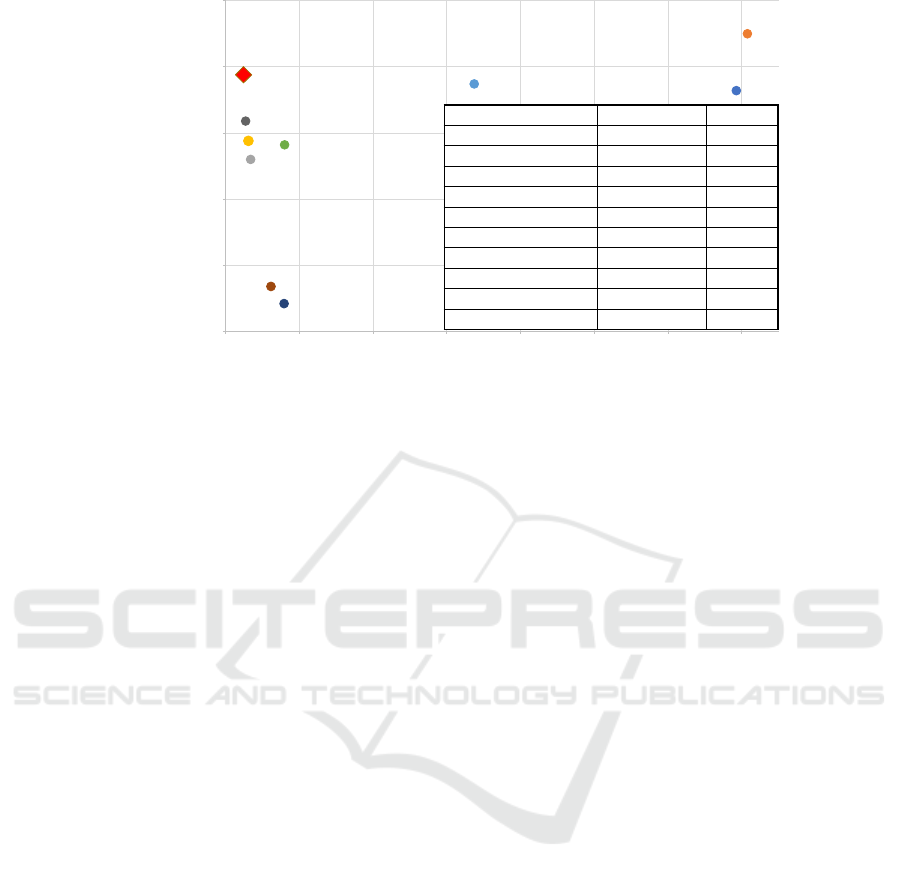
Figure 1: Model Parameters vs VOC accuracy - Lightweight SSD achieves 74.4 mAP with only 4.86M parameters on

PASCAL VOC, being 0.2x smaller yet still more accurate 3.5 mAP than the previous best lightweight detector Pelee.

This inspires us to design a new lightweight detector

named Lightweight SSD. Besides, good detectors in

mobile devices should be easy to train in less GPU.

This means Bag of freebies methods of object

detection during the detector training is

indispensable.

This paper aims to design a real-time and

lightweight detector for mobile devices.

Furthermore, this detector is easy to train in only a

few GPUs and easily used. To some extent, anyone

who uses one GPU to train and uses the mobile

device to test can achieve real-time, high quality

results, as the Lightweight SSD results are shown in

Fig.1. In summary, our contributions are two-fold:

1. We propose the innovated and efficient object

detectors Lightweight SSD. It contains a new

lightweight backbone and a new detection neck part

whose names are MBlitenet and CFPN (Circle

Feature Pyramid Networks), respectively. It makes

the detector more accurate in mobile devices and can

be trained fast in limited computation, i.e. only one

or two 2080Ti GPUs.

2. We verify the influence of “Bag of freebies”

methods of object detection during the detector

training, like Mosiac (Bochkovskiy et al., 2020),

focal loss (Lin et al., 2017). Furthermore, we

propose two new Bag of freebies methods, including

BLL (Both Localization Loss) and GrayMixRGB.

They are useful for the detector's accuracy and not

increase the operation parameters.

2 RELATED WORK

Object Detection Models: Object detection refers

to identifying whether there is an object of interest

from a new image and determining its location and

classification. Object detection models are used for

object detection, which usually includes one-stage

detectors and two-stage detectors. Standard one-

stage detectors are SSD (Liu et al., 2016), YOLO

(Redmon et al., 2016, 2017, 2018). One-stage

detector directly predicts the localization and

classification of objects from the bounding boxes in

the feature map. On the contrary, a two-stage

detector first generates a series of sparse candidate

frames on the input image through a heuristic

method or a Convolutional Neural Network. It then

extracts the feature values of these candidate frame

regions. Finally, it predicts localization and

classification of objects, such as R-FCN (Region-

based Fully Convolutional Network) (Dai et al.,

2016), Fast RCNN (Region Convolutional Neural

Network) (Girshick, 2015), Faster RCNN (Ren et

al., 2015). Intuitively, a one-stage director is an end-

to-end object detector and can realize real-time

object detection. The two-stage director's processes

are complex but have competitive accuracy. In this

work, we utilize a one-stage detector that focuses on

efficiency because of limited computing ability in a

mobile device.

Backbone Networks for Object Detection: To

design a lightweight detector, the small backbone

73.2

77.5

68

69.4

73.7

69.1

57.1

58.4

70.9

74.4

55

60

65

70

75

80

0 20406080100120140

VOC mAP

Parameters (M)

Lightweight SSD

Pelee

Mobilenet v2-SSD

YOLO Nano

Mobilenet-SSD

Tiny YOLOv3

Tiny YOLOv2

YOLOv2

Faster

R-CNN

SSD

Model Parameters mAP

Faster R-CNN 138.5 73.2

SSD300 141.5 77.5

Mobilenet-SSD300 6.8 68

Mobilenetv2-SSD 6.2 69.4

YOLOv2 67.43 73.7

YOLO Nano 16 69.1

Tiny YOLOv2 15.86 57.1

Tiny YOLOv3 12.3 58.4

Pelee 5.43 70.9

Lightweight SSD(ours) 4.86 74.4

VISAPP 2021 - 16th International Conference on Computer Vision Theory and Applications

26

networks are necessary. Some famous small

networks often are used as the backbone in light

detectors, such as Mobilenetv1/v2/v3 (Howard et al.,

2017, 2018, 2019), ShuffleNet (Zhang et al., 2018).

The Mobilenet series proposed depth separable

convolution, which decreases the computing

parameters, and the ShuffleNet proposed channel

shuffle and grouped convolution also focus on

reducing computing. Small networks for

classification or object detection's backbone part

need different attributes of networks. Therefore, it is

not appropriate to directly use a small network for

classification as the backbone of object detection. In

this work, we consider the drawbacks of previous

different lightweight backbone networks and

propose a new lightweight backbone named

MBlitenet for the lightweight detector.

Detection Neck Part for Detection Models:

Detection neck parts mainly represent feature fusion

networks, which improve detection accuracy by

fusing the feature information from multiple

different scale feature maps. Feature fusion

networks in object detection attract much research

efforts, and there are some feature fusion networks

such as FPN (Lin et al.,2017), PAN (Liu et al.,2018),

and BiFPN (Tan ET AL.,2020). FPN merges feature

information of different scales to form a feature

pyramid. PAN and BiFPN combine feature

information from a couple of feature pyramids in

order. In our work, we propose a circle feature

pyramid network (CFPN) to recycle different feature

pyramid information for fruitful feature fusion and

better object detection accuracy.

Bag of Freebies: A CNN-based object detector

contains two procedures: training and inference.

Once we have completed the training and obtained a

better model, we will use it as the inference model.

We can optimize the model to get more accuracy

and more accessible training procedure from two

aspects: training tricks and some methods only

increase training time without increasing inference

cost. The above two parts are usually called "Bag of

freebies".

The data augmentation uses some methods to

make the training dataset bigger. They have more

information dimensions for model generalization,

such as random erase (Zhong et al., 2017), CutOut

(DeVries et al.,2017), and Mosiac (Bochkovskiy et

al.,2020). In order to solve the problem of uneven

data distribution, another method in Bag of freebies

named hard negative example mining (Sung et al.,

1998) method is adopted in the training procedure.

The last Bag of freebies is designing better loss

functions, including Bounding Box regression and

classification for improving model accuracy and

easy training. Like the focal loss (Lin et al., 2017)

method, the classification loss function can balance

the negative and positive samples and consider the

classification difficulty differences. The traditional

Bounding Box regression loss function is L1 loss

function, which does not consider the intersection-

over-union (IOU) between bounding boxes and

ground truth boxes. Therefore, some new Bounding

Box regression loss functions that care about the

intersection-over-union (IOU) were proposed, such

as IOU loss (Yu et al., 2016), GIOU loss

(Rezatofighi et al., 2019). In this work, we propose

two new Bag of freebies methods, including BLL

loss and GrayMixRGB to improve detectors'

accuracy.

3 LIGHTWEIGHT SSD

Based on traditional SSD (Single Shot MultiBox

Detector), we have developed a new object detector

named Lightweight SSD. In this section, we will

discuss the detector architecture and some new parts

in this detector.

3.1 Lightweight SSD Architecture

The Lightweight SSD architecture is shown in Fig.2,

which contains three parts: the backbone, the

detection neck part, and the detection part. Fig.2

includes the Bag of freebies in the Lightweight

SSD’s training process. We proposed a new

lightweight backbone named MBlitenet for feature

extraction, and a new detection neck part named

CFPN (Circle Feature Pyramid Networks) for

feature fusion. The detection neck part takes the

level 3-7 feature maps from the backbone network

and applies the feature fusion. After that, these fused

feature maps are fed to the detection part to get the

object class and bounding box regression

respectively.

3.2 Backbone Network: MBlitenet

In this subsection, we introduce a new lightweight

backbone network named MBlitenet. The

architecture of MBlitenet is composed of both

traditional linear inverted residual bottleneck

Lightweight SSD: Real-time Lightweight Single Shot Detector for Mobile Devices

27

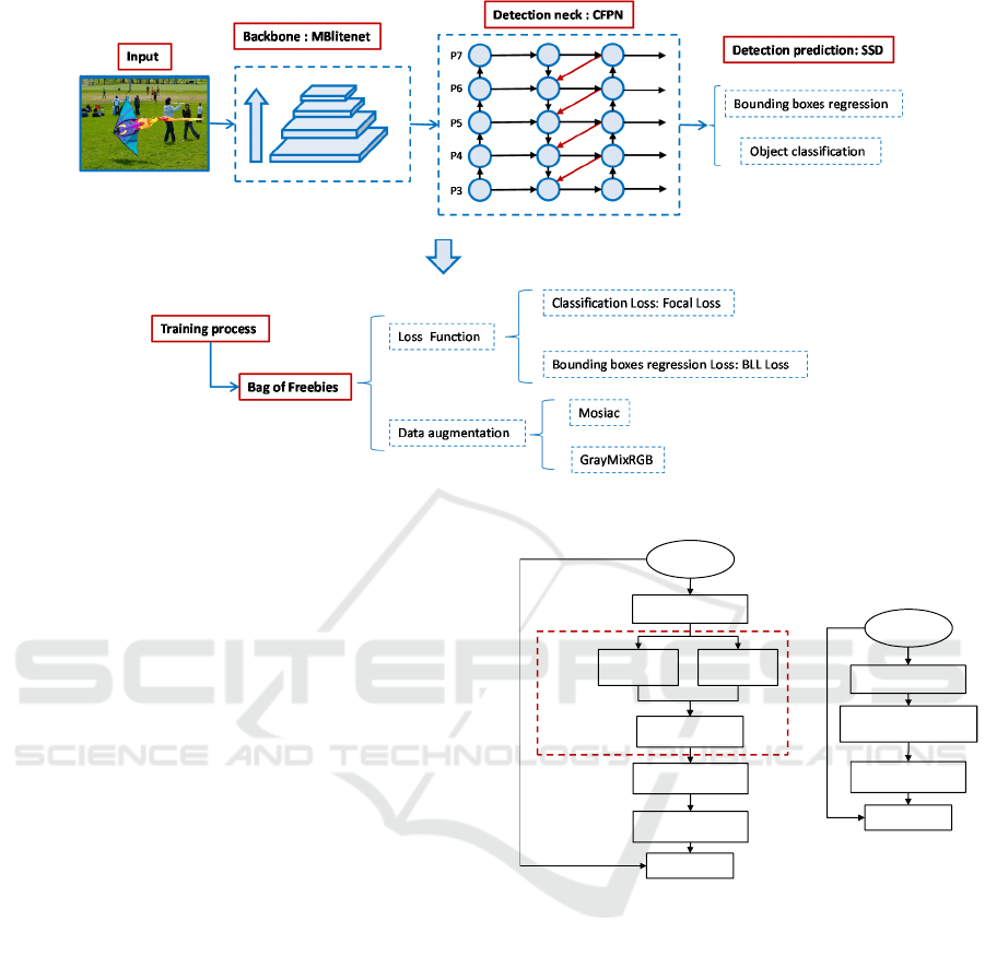
Figure 2: Lightweight SSD Architecture (above) and the Bag of freebies in Lightweight SSD’s training process (below).

(Sandler et al., 2018) and the attentive linear

inverted residual bottleneck. The detailed

convolutional operations inside these two parts are

mixed depthwise convolutions that will be

introduced in chapter 3.2.2.

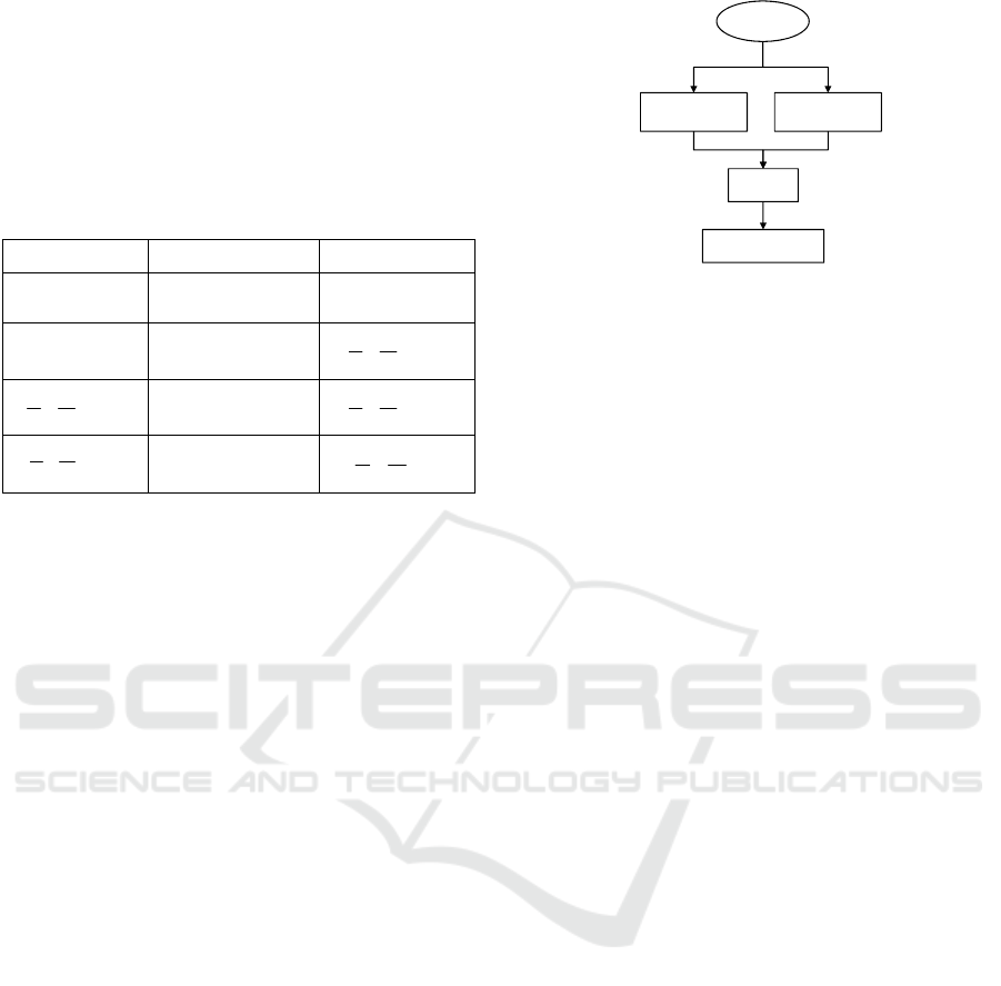
3.2.1 Attentive Linear Inverted Residual

Bottleneck

We proposed a novel part named Attentive linear

inverted residual bottleneck composed of traditional

linear inverted residual bottleneck (Sandler et

al.,2018) and spatial attention module (SAM) part

(Wang et al., 2019).

The traditional linear inverted residual

bottleneck performs feature dimensionality expend

first, and then feature dimensionality reduction

(Sandler et al., 2018). The feature maps after

dimensionality reduction use linear functions. Fig.3

shows a traditional linear inverted residual

bottleneck in the right side. The spatial attention

module part uses the pooling method to merge the

channels of feature maps. After that, get an attention

map for enhancing the original feature maps.

After adding the spatial attention module part to

the traditional linear inverted residual bottleneck,

our attentive linear inverted residual bottleneck will

focus more attention on the objected area. This

solves the problem that the traditional linear inverted

residual bottleneck does not have the spatial

attention information. And this helps the bottleneck

increase the focus on the prominent part of the

Figure 3: Attentive linear inverted residual bottleneck

(left side) and Traditional linear inverted residual

bottleneck (right side).

image, thereby improving the detector’s object

detection accuracy.

Fig.3 shows an attentive linear inverted residual

bottleneck in the left. The spatial attention module

part is used in the middle of the bottleneck. After the

mixed depthwise convolution, the spatial attention

module performs average pooling and maximum

pooling on the feature maps to obtain two 2-

dimensional images. It then merges these two

images and uses a standard convolution operation to

get the final 2-dimensional spatial attention image.

The 2-dimensional spatial attention image obtained

by the SAM module is subjected to matrix

multiplication with the original feature image. And

Conv 1ൈ1, Relu6

Input,

stride=1

Dwise 3ൈ3

Conv 1ൈ1, Linear

Add

Conv 1ൈ1, Relu6

Dwise 3ൈ3, Relu6

Conv 1ൈ1, Linear

Add

Spatial attention part

Input,

stride=1

Dwise 5ൈ5

Concat, Relu6

Mixed

Depthwise

Convolutions

VISAPP 2021 - 16th International Conference on Computer Vision Theory and Applications

28

then the new feature image obtained is used as the

input of the next pointwise convolution layer of the

network. Table 1 is the operations process of the

attentive linear inverted residual bottleneck.

Table 1: Attentive linear inverted residual bottleneck –

The dwise represent the depthwise convolution. The t

represents the expansion factor. The k and k’ represent the

output channels and s represents stride.

Input Operation Output

hwk××

1x1 conv2d，

ReLU

()hw tk××

3x3,5x5dwise,

ReLU

()

hw

tk

s

××

()

hw

tk

s

××

spatial attention

module

()

hw

tk

s

××

()

hw

tk

s

××

Linear 1x1

conv2d

'

hw

k

s

××

3.2.2 Mixed Depthwise Separable

Convolutions

Depthwise Separable Convolutional is an efficient

block for many lightweight neural network

architectures (Howard et al., 2017). Therefore, we

use it as a fundamental convolution part of the

present work. Depthwise Separable Convolutional

includes depthwise convolution and pointwise

convolution two parts. The depthwise convolution

part applies a single convolutional filter per input

channel to realize lightweight. The pointwise

convolution is 1×1 convolution, which is used to

fuse the features through different channels after

depthwise convolution.

Furthermore, to facilitate our module to get a

larger receptive field, we use Mixed Convolution

(Tan et al.,2019) to replace the traditional depthwise

convolution in Depthwise Separable Convolution,

and called this new convolution operation Mixed

Depthwise Separable Convolution. The architecture

of Mixed Depthwise Separable Convolution is in

Fig.4. Mixed Convolution means not only use one

size kernel filter but apply kinds of different kernel

sizes to get a larger receptive field. In this paper, we

apply both 3×3 and 5×5 kernel filters in mixed

depthwise convolution. The operation is splitting the

input tensor into two parts in channels, and one part

uses 3×3 kernel's depthwise convolution. The other

part uses 5×5 kernel's depthwise convolution.

Finally, we merge these two parts to finish mixed

depthwise convolution.

Figure 4: Mixed Depthwise Separable Convolution.

Standard convolution gets an input

tensor

,

II

D

DM××

and the output tensor

is

II

D

DN××

. The kernel size is

.

KK

D

DMN×××

The computation cost of standard convolution is

I

IKK

DDMND D×××× ×

.

In the same situation, the Mixed Depthwise

Separable Convolution has two steps. Firstly, mixed

depthwise convolution part’s computation cost is

equation (1):

11 2 2

/2 + /2

=/2

I

IKKIIKK

II K K K K

D

DM D D DDM D D

DDM DDDD

×× × × ×× × ×

×× × × + ×（

）

(1)

Next, the pointwise convolution part’s

computation cost is equation (2):

11

II

DD MN×××××

(2)

The computation cost of Mixed Depthwise

Separable Convolution is equation (3):

11 2 2

/2

II K K K K II

D

DM D D D D DDM

N

×× × × + × +×××（）

(3)

From the equations, it is clear that the Mixed

Depthwise Separable Convolution is 7~8 times less

computation than the standard convolution.

3.2.3 MBlitenet Architecture

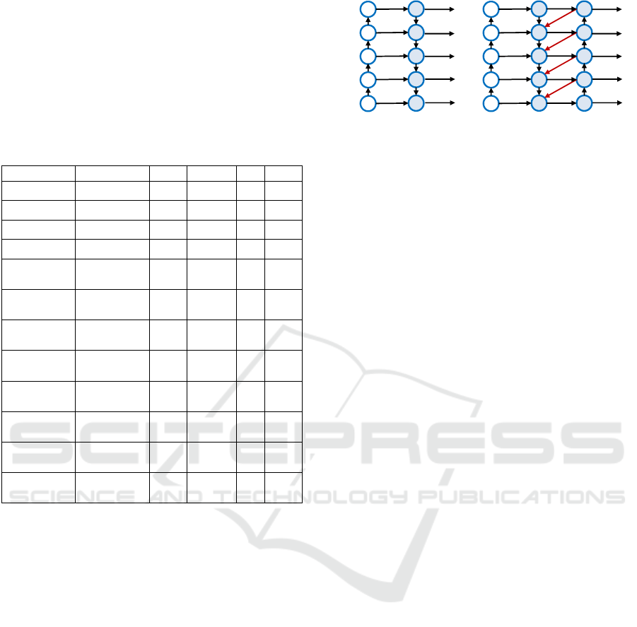
Only one kind of bottleneck cannot fully utilize the

feature extraction capabilities of the model.

Therefore, the architecture of MBlitenet is in Table

2, which is composed of a traditional linear inverted

residual bottleneck, mixed linear inverted residual

bottleneck, and attentive linear inverted residual

bottleneck. Traditional linear inverted residual

bottleneck and attentive linear inverted residual

bottleneck have been introduced in chapter 3.2.1.

The mixed linear inverted residual bottleneck only

Input

Dwise 5ൈ5

concat

Dwise 3ൈ3

Conv 1ൈ1

Lightweight SSD: Real-time Lightweight Single Shot Detector for Mobile Devices

29

replaces the Depthwise Separable Convolutional in

traditional linear inverted residual bottleneck to the

Mixed Depthwise Separable Convolution.

Table 2: MBlitenet architecture - Each line represents a

bottleneck or a regular convolution, repeated n times. The

c represents the output channels of each layer. The first

layer of each bottleneck has a stride s and all others use

stride 1. The t represents the expansion factor of each

bottleneck.

Input Operation t c n s

2

300 3×

conv2d - 64 1 1

2

300 64×

conv2d - 32 1 2

2

150 32×

bottleneck 1 16 1 1

2

150 16×

bottleneck 6 24 2 2

2

75 24×

attentive-

bottleneck

6 32 3 2

2

38 32×

mix-

bottleneck

6 64 4 2

2

19 64×

attentive-

bottleneck

6 96 3 1

2

10 96×

mix-

bottleneck

6 160 3 2

2

5160×

attentive-

bottleneck

6 320 1 1

2

5 320×

conv2d

1x1

- 1280 1 1

2

5 1280×

Avgpool

5x5

- - 1 -

2

1 1280×

Conv2d

1x1

- k -

3.3 Detection Neck Part: CFPN

Based on the traditional FPN (Feature Pyramid

Networks) (Lin et al., 2017), and think about the

actual biological neuron connection process, a

specific neuron between different neurons may be the

input or output node other neurons. We proposed a

new CFPN (Circle Feature Pyramid Networks) that

circularly fuses the feature information so that

different scales' feature information is better

integrated.

The circle feature fusion network of CFPN and

traditional FPN are shown in Fig.5(b) and Fig.5(a),

respectively. The purpose of CFPN is to fuse feature

information of different feature maps scales.

As shown in Fig.5 (b),

34 7

( , ,..., )

in in in in

P

PP P=

represents the level of 3-7 feature maps from

backbone network, and intermediate fusion layer is

34 7

( , ,..., )

mid mid mid mid

PPPP=

. Finally, the output feature

maps from CFPN is

34 7

(,,...,)

out out out out

PPPP=

.

Figure 5: FPN and CFPN feature fusion networks.

The procedure of CFPN (Circle Feature Pyramid

Networks) is as follows equation (4):

77

66 7 7

33 4 4

Resize( ) Resize( )

...

Resize( ) Resize( )

mid in

mid in mid out

PP

PP P P

=

=+ +

(4)

After obtaining the intermediate layer result, the

final output feature fusion result is obtained from the

intermediate layer result:

77 6

66 5

33

( Resize( ))

(Resize())

...

()

out mid out

out mid mid

out mid

P Conv P P

P Conv P

=+

=

(5)

where Resize is usually upsampling or

downsampling for resolution matching, and Conv is

usually convolution for feature processing.

3.4 Bag of Freebies: BLL Loss and

GrayMixRGB

3.4.1 BLL (Both Localization Loss) Loss

The traditional SSD object detection algorithm's loss

function contains two parts: classification loss and

position regression loss.

The classification loss function has been

optimized for Focal loss. For the position regression

loss function, the traditional object detection

algorithms usually use the Smooth L1 loss function.

However, in the evaluation of the detection boxes,

the IOU (Intersection over Union) is used to

evaluate the prediction box's quality compared with

the ground truth box. The Smooth L1 loss and the

value of IOU are not equivalent. To solve this

problem, Jiahui Yu et al. (Yu et al., 2016) proposed

IoU Loss in 2016. However, IoU Loss keeps zero

when the prediction box and the ground truth box do

not intersect. It cannot reflect the distance between

P3

P4

P5

P6

P7

P3

P4

P5

P6

P7

(a) FPN (b) CFPN

VISAPP 2021 - 16th International Conference on Computer Vision Theory and Applications

30

the prediction box and the ground truth box, and it

cannot be derived at this time.

To solve the above-mentioned problems of IoU

Loss, Zhaohui Zheng et al. proposed DIoU Loss and

CIoU Loss (Zheng et al.,2020) in 2020. The formula

of DIoU Loss is defined as follows equation (6):

2

(,)

1

ab

DIoU loss IoU

c

ρ

=− +

(6)

Where,

ρ

represents the Euclidean distance, a,b

represents the center point of the prediction box and

ground truth box respectively, c represents the

diagonal distance of the smallest bounding rectangle

of the prediction box A and the ground truth box B.

The formula of CIoU Loss is defined as follows

equation (7):

2

(,)

1

(1 )

4

(arctan arctan )

gt

ab

CIoU loss IoU v

c

v

IoU v

ww

v

hh

ρ

α

π

=− + +

=

−+

=−

(7)

Where,

g

t

w

and

g

t

h

represent the width and

height of the ground truth box respectively, w and h

represent the width and height of the predicted box.

Regarding the IoU Loss, DIoU Loss, and CIoU

Loss mentioned above, observing their formulas, we

can see that their formulas have common points.

They all contain

1

I

oU−

part, mainly for the overlap

area of the ground truth box and the predicted box.

The formula’s last part focuses on the center point

distance or aspect ratio between the ground truth

box and the predicted box. In the position regression

loss function, the center point distance and aspect

ratio between the ground truth box and the predicted

box is the part that the traditional Smooth L1 loss

function or L2 loss function are concerned about.

Therefore, we innovatively propose the

BothLocalizationLoss (BLL) position regression

loss function. Considering the overlap area, center

point distance, and aspect ratio of the ground truth

box and the predicted box, the formula is simplified

as much as possible to facilitate practical application

and implementation. The formula is defined as

follows equation (8):

2

1

Lloss

BothLocalizationLoss IoU

c

=− +

(8)

Where, c represents the diagonal distance of the

smallest bounding rectangle of the prediction box

and the ground truth box.

2

c

helps unify the

2

L

loss

and

1

I

oU−

to the similar values.

The formula contains both the

1

I

oU−

part to

focus on the overlapping area of the prediction box

and the ground truth box, and the Smooth L1 loss

function or the L2 loss function, which is used to

focus on the center point distance and aspect ratio

between the ground truth box and the predicted box.

The most crucial point is that compared with

CIoU Loss, it dramatically reduces the complexity

of the formula and the complexity of the

implementation code, making it more suitable for

multiple applications in the actual field.

3.4.2 Data Augmentation: GrayMixRGB

In this section, we will perform a new data

augmentation method named GrayMixRGB. As we

all know, the color image and grayscale image of the

same picture contain the same objects. This is very

easy to recognize for humans. However, it is

difficult for the CNN-detector model to maintain the

model's robustness, enabling the model to recognize

the same target under both grayscale and color

images. In order to solve this problem, we propose

this new data augmentation method GrayMixRGB.

It can make the training set images contain the color

information and gray information at the same time.

The process of GrayMixRGB dealing with the

training set images is three steps: Firstly, getting an

image from the training set. Secondly, replacing the

minimum value from the image’ RGB values to the

gray value. Finally, save the new image. The

program code of this process is as follows:

begin

img = RGBimage

imggray = grayimage

height = img’s height

width = img’s width

for i,j in range height,width:

for k in range(3):

# find the minimum value of RGB

if img[i,j,k] < min:

min=minimum of RGB

index=index of minimum

if imggray[i,j] > min:

# change minimum to gray value

img[i,j,index]=imggray[i,j]

End.

3.4.3 Additional Bag of Freebies: Mosaic

We innovatively combine the Mosaic data

augmentation method used in YOLOv4

(Bochkovskiy et al., 2020). Mosaic is a data

augmentation method by mixing 4 training images.

The example is shown in Fig.6. It also mixes the

semantics of the four images simultaneously. The

Lightweight SSD: Real-time Lightweight Single Shot Detector for Mobile Devices

31

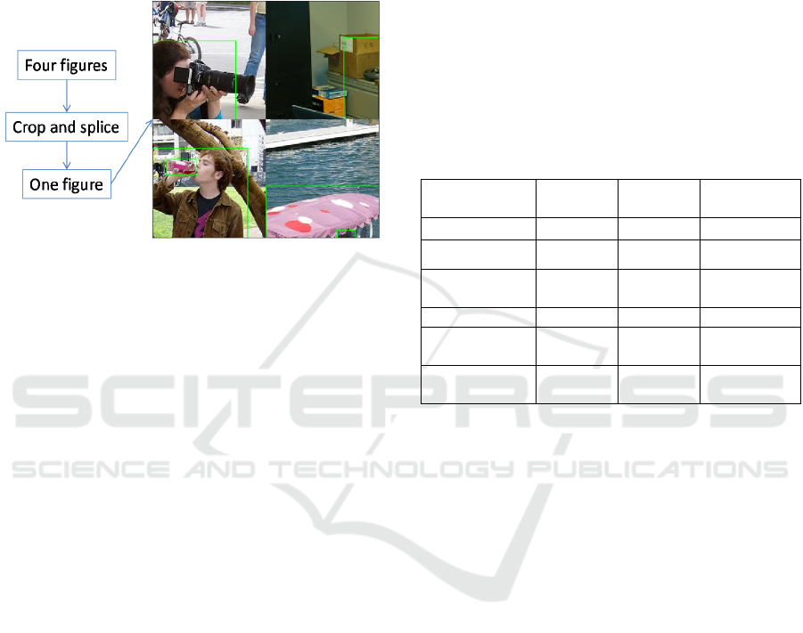
purpose is to make the detected targets exceed their

general semantics and make the model have better

robustness. Simultaneously, doing Mosiac enables

the batch normalization (BN) operation during

training to count 4 images at a time, which can

sufficiently reduce the size of the largest mini-batch

during training.

Figure 6: Mosaic data augmentation method.

4 EXPERIMENTS

In this section, we first evaluate the effects of our

proposed backbone MBlitenet and the CFPN part

with SSD detectors on both MS COCO (test-dev

2017) dataset (Lin et al., 2014) and PASCAL VOC

(07+12trainval and 07 test) dataset (Everingham et

al.,2010). We then show the performance of the

other parts of Lightweight SSD on VOC

(07+12trainval and 07test) dataset. Finally, we

compare our Lightweight SSD detector to other

lightweight detectors on VOC (07+12trainval and

07test) dataset. The deep learning platform uses

Tensorflow.

4.1 Evaluation Effect of Backbone and

the CFPN

In this paper, we proposed the backbone MBlitenet

and the detection neck part CFPN in Lightweight

SSD detector. We expect to know how much each of

them can contribute to the detector’s accuracy and

efficiency. Table 3 compares the effect of the

backbone MBlitenet and the CFPN in both COCO

and VOC dataset. All backbone and detection neck

part in Table 3 are based on SSD detector. Starting

from the backbone part, our proposed MBlitenet’s

accuracy is 1.1 mAP better than Mobilenet v2

(Sandler et al., 2018) and 2.5 mAP better than

Mobilenet (Howard et al., 2017) in VOC dataset

with slightly less parameters. This means the

MBlitenet is a better backbone with both good

accuracy and lightweight for mobile device. At the

same time, our proposed detection neck part CFPN’s

accuracy is 1.1 mAP better than traditional FPN (Lin

et al.,2017) method and 3.5 mAP better than no use

feature fusion method. These results suggest that the

MBlitenet backbone and the CFPN detection neck

part are both essential to our final lightweight

Lightweight SSD detector in mobile device.

Table 3: Evaluation effect of Backbone and the CFPN in

COCO and VOC - The mAP (VOC) represents the mAP

results in VOC dataset. The mAP (COCO) represents the

mAP results in COCO dataset. The “-” means no relevant

data.

mAP

(VOC)

mAP

(COCO)

Parameters

Mobilenet

68 19.3 6.8M

Mobilenet v2

69.4 21.5 6.2M

Mobilenet v2

+ FPN

71.9 - 6.6M

MBlitenet

70.5

22.3 4.16M

MBlitenet

+ FPN

72.9 - 4.6M

MBlitenet

+ CFPN

74

- 4.86M

4.2 Evaluation Effect of the Bag of

Freebies

In this paper, we proposed two Bag of freebies

methods and apply Mosiac method to our detector.

We need to evaluate how effective these methods

are for our Lightweight SSD detector. The Bag of

freebies will not affect the parameters of the

detectors, but only affect the accuracy. Therefore, in

the comparison experiment, we only focus on

accuracy of the detectors. Table 4 compares the

effect of different Bag of freebies used in the

Lightweight SSD detector on VOC dataset. The

basic Lightweight SSD detector contains the

MBlitenet backbone, the CFPN detection neck part,

and the SSD prediction part. Table 4 shows that

after applying BLL Loss as the localization

regression loss, the accuracy is improved 0.1 mAP

in VOC dataset.

After applying GrayMixRGB data augmentation,

the accuracy is improved 0.2 mAP than the basic

Lightweight SSD in VOC dataset. The BLL Loss

helps the prediction bounding boxes position more

exact, and the GrayMixRGB data augmentation

makes the dataset contain the gray information that is

VISAPP 2021 - 16th International Conference on Computer Vision Theory and Applications

32

Table 5: Lightweight SSD performance on PASCAL VOC.

Model Backbone Input Parameters mAP

Faster R-CNN

VGG-16 300*300 138.5M 73.2

SSD300

VGG-16 300*300 141.5M

77.5

SSD300

Mobilenet 300*300 6.8M 68

SSD300

Mobilenet v2 300*300 6.2M 69.4

SSD300

Mobilenet v2

+ FPN

300*300 6.6M 71.9

YOLOv2

Darknet-19 544*544 67.43M 73.7

YOLOv3

Darknet-53 608*608 62.3M 84.1

YOLOv3

Mobilenet 300*300 - 66

YOLO Nano

- 300*300 16M 69.1

Tiny YOLOv2

Tiny Darknet 416*416 15.86M 57.1

Tiny YOLOv3

Tiny Darknet 416*416 12.3M 58.4

ThunderNet

SNet49 320*320 - 70.1

Pelee

PeleeNet 304*304 5.43M 70.9

Lightweight

SSD(ours)

MBlitenet

+ CFPN

300*300

4.86M 74.4

better for the detector's robustness. However, the

Mosaic data augmentation does not perform well in

our detector. The reason is that some images after

the Mosaic data augmentation will only contain

some meaningless ground truth boxes but not real

semantic objects in the boxes.

Table 4: Evaluation effect of the Bag of freebies in

PASCAL VOC – The “” represents the Lightweight

SSD detector apply this Bag-of-Freebie. The “ - ”

represents the Lightweight SSD detector does not apply

this Bag-of-Freebie.

BLL Loss GrayMixRGB Mosaic mAP

- - - 74



- - 74.1

-



- 74.2

- -



72.7

 

-

74.4

4.3 Lightweight SSD for Object

Detection

We evaluate our Lightweight SSD on PASCAL

VOC dataset, which contains the 12+07 trainval data

as our training set and 07 test data as our test

dataset. The results are exhibited in Table 5. The

model is trained using Momentum optimizer with

momentum 0.9 and with batch size 126 on 3 Nvidia

GeForce RTX 2080 Ti GPUs. The learning rate is

the cosine decay learning rate with the base learning

rate 0.1, warm up learning rate 0.0333, and the total

steps are 500k. For the activation function, we use

the ReLU activation. We also apply commonly-used

focal loss with

=0.25

α

and

=2.0

γ

.

Lightweight SSD exceeds the previous state-of-

the-art lightweight detectors. Lightweight SSD

achieves 74.4 mAP with only 4.86M parameters on

PASCAL VOC, being nearly 30% smaller than the

Mobilenet-SSD and surpassing Mobilenet-SSD

(Wang et al.,2018) by 6.4 mAP. The Lightweight

Lightweight SSD: Real-time Lightweight Single Shot Detector for Mobile Devices

33

SSD also performs better than the Tiny YOLO-

series by almost 6 mAP and lighter 50% than Tiny

YOLO-series (Redmon et at., 2017). Moreover,

Lightweight SSD performs better than the two-stage

detector ThunderNet (Qin et al., 2019) by 4.3 mAP.

As a result, Lightweight SSD is 0.2x smaller yet still

more accurate 3.5 mAP than the previous best

lightweight detector Pelee (Wang et al., 2018).

Furthermore, the Lightweight SSD achieves a

competitive accuracy to the state-of-art large

detectors such as YOLOv2 (Redmon et at., 2017),

Faster R-CNN (Liu et al., 2016), and SSD300 (Liu

et al., 2016), but really decreases the computation

cost.

The models’ inference speed in Table 6 is

obtained in only 1 Nvidia GeForce RTX 2080 Ti

GPU, which can represent the mobile devices with

the edge ASIC. Because the edge ASIC means the

GPU specially designed for the mobile device

Table 6: The speed for different model on RTX 2080 Ti -

The speed represents that the detector infers one image’s

time.

Model Backbone Input Speed

(ms)

SSD300 Mobilenet 300*300

23

SSD300 Mobilenet v2 300*300 23.5

SSD300 Mobilenet v2

+ FPN

300*300 24

YOLOv3 Darknet-53 608*608 46

Lightweight

SSD(ours)

MBlitenet

+ CFPN

300*300 23.7

From the Table 5 and the Table 6, the

Lightweight SSD is compared to a lot of previous

detectors in accuracy, parameters and speed. It

performs a much better balance between accuracy

and computation cost. Lightweight SSD is a very

efficient detector to apply on practical mobile

devices.

5 CONCLUSIONS

This paper proposes a lightweight and efficient

object detector named the Lightweight SSD for

mobile devices. In the backbone part, we analyse

past lightweight backbone networks and design our

MBlitenet backbone based on their advantages and

circumvent their shortcomings. In the detection neck

part, we propose an efficient feature fusion network

CFPN. Two innovative and useful Bag of freebies

named BLL loss and GrayMixRGB are applied to

the Lightweight SSD detector to further improve

detector capabilities and efficiency without

increasing the inference computation. Lightweight

SSD achieves a very competitive accuracy with

particularly less computational cost in mobile

devices. We hope to consider an efficient object

detector for both arm and edge ASIC model devices

in the future.

REFERENCES

Kaiming He, Xiangyu Zhang, Shaoqing Ren, Jian Sun.

(2015). Deep Residual Learning for Image

Recognition. In Computer Vision and Pattern

Recognition, 2015. CVPR 2015, abs/1512.03385.

Andrew G. Howard, Menglong Zhu, Bo Chen,Dmitry

Kalenichenko, Weijun Wang, Tobias Weyand, Marco

Andreetto, and Hartwig Adam. (2017). Mobilenets:

Efficient convolutional neural networks for mobile

vision applications. In Computer Vision and Pattern

Recognition, 2017. CVPR 2017, abs/1704.04861.

T. Lin, P. Doll´ar, R. B. Girshick, K. He, B. Hariharan, S.

J. Belongie. (2017). Feature pyramid networks for

object detection. In Computer Vision and Pattern

Recognition, 2017. CVPR 2017, abs/1807.03284.

Shu Liu, Lu Qi, Haifang Qin, Jianping Shi, and Jiaya Jia.

(2018). Path aggregation network for instance

segmentation. In Proceedings of the IEEE Conference

on Computer Vision and Pattern Recognition,2018.

CVPR 2018, pages 8759–8768.

Wei Liu, Dragomir Anguelov, Dumitru Erhan, Christian

Szegedy, Scott Reed, Cheng-Yang Fu, and Alexander

C Berg. (2016). SSD: Single shot multibox detector.

In Proceedings of the European Conference on

Computer Vision (ECCV), 2016, pages 21–37.

Joseph Redmon, Santosh Divvala, Ross Girshick, and Ali

Farhadi. (2016). You only look once: Unified, real-

time object detection. In Proceedings of the IEEE

Conference on Computer Vision and Pattern

Recognition (CVPR),2016, pages 779–788.

Joseph Redmon, Ali Farhadi. (2017). YOLO9000: better,

faster, stronger. In Proceedings of the IEEE

Conference on Computer Vision and Pattern

Recognition (CVPR),2017,pages 7263–7271.

Joseph Redmon and Ali Farhadi. (2018). YOLOv3: An

incremental improvement. arXiv, preprint

arXiv:1804.02767.

Alexey Bochkovskiy, Chien-Yao Wang, Hong-Yuan

Mark Liao. (2020). YOLOv4: Optimal Speed and

Accuracy of Object Detection. In Proceedings of the

IEEE Conference on Computer Vision and Pattern

Recognition (CVPR),2020, arXiv:2004.10934.

Tsung-Yi Lin, Priya Goyal, Ross Girshick, Kaiming He,

Piotr Doll´ar. (2017). Focal loss for dense object

detection. In Proceedings of the IEEE International

VISAPP 2021 - 16th International Conference on Computer Vision Theory and Applications

34

Conference on Computer Vision (ICCV),2017, pages

2980–2988.

Jifeng Dai, Yi Li, Kaiming He, and Jian Sun. (2016). R-

FCN:Object detection via region-based fully

convolutional networks. In Advances in Neural

Information Processing Systems (NIPS),2016, pages

379–387.

Ross Girshick. (2015) Fast R-CNN. In Proceedings of the

IEEE International Conference on Computer Vision

(ICCV), 2015,pages 1440–1448.

Shaoqing Ren, Kaiming He, Ross Girshick, and Jian Sun.

(2015).Faster R-CNN: Towards real-time object

detection with region proposal networks. In Advances

in Neural Information Processing Systems (NIPS),

2015,pages 91–99.

Xiangyu Zhang, Xinyu Zhou, Mengxiao Lin, and Jian Sun.

(2018). ShuffleNet: An extremely efficient

convolutional neural network for mobile devices. In

Proceedings of the IEEE Conference on Computer

Vision and Pattern Recognition (CVPR), 2018, pages

6848–6856.

Mark Sandler, Andrew G. Howard, Menglong Zhu,

Andrey Zhmoginov, and Liang-Chieh Chen. (2018).

Mobilenetv2: Inverted residuals and linear bottlenecks.

mobile networks for classification, detection and

segmentation. In the IEEE Conference on Computer

Vision and Pattern Recognition (CVPR), 2018, pp.

4510-4520.

Andrew Howard, Mark Sandler, Grace Chu, Liang-Chieh

Chen, Bo Chen, Mingxing Tan, Weijun Wang, Yukun

Zhu, Ruoming Pang, Vijay Vasudevan. (2019).

Searching for mobilenetv3. In Proceedings of the

IEEE International Conference on Computer Vision

ICCV, 2019, arXiv:1905.02244.

Mingxing Tan, Ruoming Pang, and Quoc V Le. (2020).

EfficientDet: Scalable and efficient object detection.

In Proceedings of the IEEE Conference on Computer

Vision and Pattern Recognition (CVPR), 2020.

Zhun Zhong, Liang Zheng, Guoliang Kang, Shaozi Li,

and Yi Yang. (2017). Random erasing data

augmentation. ArXiv preprint arXiv:1708.04896, 2017.

Terrance DeVries and Graham W Taylor. (2017).

Improved regularizationb of convolutional neural

networks with CutOut. arXiv preprint

arXiv:1708.04552, 2017.

K-K Sung and Tomaso Poggio. (1998). Example-based

learning for view-based human face detection. IEEE

Transactions on Pattern Analysis and Machine

Intelligence (TPAMI),1998, 20(1):39–51.

Jiahui Yu, Yuning Jiang, Zhangyang Wang, Zhimin Cao,

and Thomas Huang. (2016). UnitBox: An advanced

object detection network. In Proceedings of the 24th

ACM international conference on Multimedia, 2016,

pages 516–520.

Hamid Rezatofighi, Nathan Tsoi, JunYoung Gwak, Amir

Sadeghian, Ian Reid, and Silvio Savarese. (2019).

Generalized intersection over union: A metric and a

loss for bounding box regression. In Proceedings of

the IEEE Conference on Computer Vision and Pattern

Recognition (CVPR), 2019, pages 658–666.

TiancaiWang, Rao Muhammad Anwer, Hisham Cholakkal,

Fahad Shahbaz Khan, Yanwei Pang, and Ling Shao.

(2019). Learning rich features at high-speed for

single-shot object detection. In Proceedings of the

IEEE International Conference on Computer Vision

(ICCV), 2019, pages 1971–1980.

Mingxing Tan, Quoc V. Le. (2019). MixConv: Mixed

Depthwise Convolutional Kernels. In the British

Machine Vision Conference (BMVC), 2019,

arXiv:1907.09595.

Zhaohui Zheng, Ping Wang, Wei Liu, Jinze Li,

Rongguang Ye, and Dongwei Ren. (2020). Distance-

IoU Loss: Faster and better learning for bounding box

regression. In Proceedings of the AAAI Conference on

Artificial Intelligence (AAAI), 2020.

Tsung-Yi Lin, Michael Maire, Serge Belongie, James

Hays, Pietro Perona, Deva Ramanan, Piotr Doll´ar,

and C Lawrence Zitnick. (2014). Microsoft COCO:

Common objects in context. In Proceedings of the

European Conference on Computer Vision

(ECCV),2014.

M. Everingham, L. Van Gool, C. K. Williams, J. Winn,

and A. Zisserman. (2010). The pascal visual object

classes (voc) challenge. International journal of

computer vision, 2010,88(2):303–338.

Zheng Qin, Zeming Li, Zhaoning Zhang, Yiping Bao,

Gang Yu, Yuxing Peng, Jian Sun. (2019). ThunderNet:

Towards Real-time Generic Object Detection. In

Proceedings of the IEEE Conference on Computer

Vision and Pattern Recognition (CVPR),2019,

arXiv:1903.11752.

R. J. Wang, X. Li, and C. X. Ling. (2018). Pelee: a real-

time object detection system on mobile devices. In

Advances in Neural Information Processing Systems,

2018, pages 1963–1972.

Lightweight SSD: Real-time Lightweight Single Shot Detector for Mobile Devices

35