PRAQA: Protein Relative Abundance Quantiﬁcation Algorithm

for 3D Fluorescent Images

Corrado Ameli

1,4 a

, Sonja Fixemer

1,2 b

, David S. Bouvier

1,2,3 c

and Alexander Skupin

1,5 d

Luxembourg Centre for Systems Biomedicine, University of Luxembourg, Luxembourg

Luxembourg Centre for Neuropathology, Laboratoire National de Sant

e, Dudelange, Luxembourg

National Center of Pathology, Laboratoire National de Sant

e, Dudelange, Luxembourg

Universit

a degli Studi di Milano, Milan, Italy

University California San Diego, La Jolla, U.S.A.

Keywords:

Confocal Fluorescent Microscopy, Image Processing, Protein Quantiﬁcation, Alzheimer’s Disease, Lewy

Body Dementia.

Abstract:

In confocal ﬂuorescent microscopy, the quality of the acquisition strongly depends on diverse factors including

the microscope parameterization, the light exposure time, the type and concentration of the antibodies used,

the thickness of the sample and the degradation of the biological tissue itself. All these factors critically

inﬂuence the ﬁnal result and render tissue protein quantiﬁcation challenging due to intra- and inter-sample

variability. Therefore, image processing techniques need to address the acquisitions variability to minimize the

risk of bias coming from changes in signal intensity, noise and parameterization. Here, we introduce Protein

Relative Abundance Quantiﬁcation Algorithm (PRAQA), a 1-parameter based, fast and adaptive approach for

quantifying protein abundance in 3D ﬂuorescent-immunohistochemistry stained tissues that requires no image

preprocessing. Our method is based on the assessment of the global pixel intensity neighborhood dispersion

that allows to statistically infer whether each small region of an image can be considered as positive signal

or background noise. We benchmark our method with alternative approaches from literature and validate its

applicability and efﬁciency based on synthetic scenarios and a real-world application to post-mortem human

brain samples of Alzheimer’s Disease and Lewy Body Dementia patients. PRAQA is implemented in Matlab

and freely available at https://doi.org/10.17881/j20h-pa27.

1 INTRODUCTION

Life relies on the proper function of its essential build-

ing blocks, the cells (Alberts, 2017). The functional-

ity of cells is ensured by the orchestrated action of

a plethora of molecules where in particular proteins

encoded by genes are essential for structure, func-

tion and regulation. Impairment in protein functions

caused by mutations in the encoding genes or by ex-

ternal perturbations often result in perturbed regula-

tory mechanisms and subsequent changes in protein

abundance which in turn may trigger different dis-

eases including cancer, diabetes and neurodegener-

ation. To investigate underlying regulatory disease

https://orcid.org/0000-0002-9101-0890

https://orcid.org/0000-0002-2312-6947

https://orcid.org/0000-0002-8630-1044

https://orcid.org/0000-0002-8955-8304

mechanisms, it is therefore essential to characterize

protein abundance and localization also in the context

of cellular heterogeneity (Komin and Skupin, 2017).

Immunostaining methods, including immunoﬂu-

orescence, revolutionized the scientiﬁc world by ex-

ploiting antibody speciﬁcities to target and visual-

ize antigens of interest in biological tissues by mi-

croscopy (Im et al., 2019). This technique allows

for estimating the distribution and the quantiﬁcation

of targeted proteins at the microscopic scales, which

are essential for assessing the roles of proteins or cel-

lular and subcellular alterations in pathological con-

ditions. A general challenge is thereby the post-

acquisition analysis of microscopy images for which

different methods have been developed as compre-

hensively discussed in (Varghese et al., 2014).

In ﬂuorescent microscopy, a common drawback of

these methods is the typical need of a preprocessing

step to transform the image into an appropriate in-

Ameli, C., Fixemer, S., Bouvier, D. and Skupin, A.

PRAQA: Protein Relative Abundance Quantiﬁcation Algorithm for 3D Fluorescent Images.

DOI: 10.5220/0010187400210030

In Proceedings of the 14th International Joint Conference on Biomedical Engineering Systems and Technologies (BIOSTEC 2021) - Volume 2: BIOIMAGING, pages 21-30

ISBN: 978-989-758-490-9

put format fulﬁlling requirements such as background

uniformity or noise reduction, or the dependence of

more than one tuning parameter in order to achieve

the quantiﬁcation. The wide range of options for

parameterizing has the advantage that the quantiﬁ-

cation procedure can be adapted to different imag-

ing conditions but irremediably increases the proce-

dure complexity and subsequently leads to potential

biases originated by an inaccurate choice of methods

or parameters. While deep-learning methods are able

to provide parameter-free analysis, the adaptability

to a plethora of acquisition conditions requires huge

amount of data to train the network (Belthangady and

Royer, 2018). This requirement cannot always be sat-

isﬁed, particularly for limited sample availability such

as for human brain samples.

Furthermore, advances in high-resolution ﬂuores-

cent microscopy now allow for processing of thicker

samples in the range of 50 to several hundreds of mi-

crometers. Larger 3D acquisitions have higher infor-

mation content but, on the other hand, they are af-

fected by larger signal intensity variability caused by

the thickness of the section (Chung et al., 2013; Bou-

vier et al., 2016) that makes reliable and robust quan-

tiﬁcation challenging.

To address these challenges, we here introduce

PRAQA (Protein Relative Abundance Quantiﬁ-

cation Algorithm), that is optimized for protein

quantiﬁcation in 3D ﬂuorescent confocal tile scan

microscope acquisitions. With only one parameter

and no preprocessing required, PRAQA is easy to

use, fast and extremely resilient to intensity changes

as well as robust for noise compromised images. We

benchmark PRAQA against alternative approaches

in synthetic scenarios and test its efﬁciency by

an application to paraformaldehyde ﬁxed human

brain samples in the context of neurodegeneration

representing a challenging scenario due to extreme

inter- and intra-sample variability.

The manuscript is organised as follows:

• Section 2 describes the algorithm and its imple-

mentation.

• Section 3 presents two synthetic scenarios and

benchmarks PRAQA with alternative algorithms

from literature.

• Section 4 presents an application on a real sce-

nario.

• Section 5 discusses advantages and drawbacks of

PRAQA and points to future work.

2 METHODOLOGY

The different sources of variability mentioned above

render a robust correction challenging and practically

impossible. Hence, image processing aims at solving

the parallel problem of an image binarization obeying

invariance with respect to the overall signal power.

PRAQA is approaching this challenge by a statisti-

cal test based on Median Absolute Deviation (MAD)

to reliably distinguish background noise from ﬂuores-

cent signal among images with different contrast.

The advantage of MAD compared to other dis-

persion or outlier detection methods is its robustness

with respect to extreme values (Leys et al., 2013) and

is therefore an appropriate choice for binarization.

PRAQA classiﬁes pixels as positive when the neigh-

borhood average intensity exceeds θ scaled MAD

where the scaled MAD of a vector x is determined

MAD

(x) =

− med(x)

med(

− med(x)

)

(1)

with med(x) being the median of the vector x.

In Section 3.3, we empirically evaluate the robust-

ness of θ with respect to different signal strengths.

2.1 PRAQA Pseudocode

The implementation of PRAQA is described in the

following by pseudocode and corresponding expla-

nations. For a given 3D image I and a threshold θ,

PRAQA calls the binarizeMAD function:

1 function binarizeMAD(I,theta)

2 I = I./max(I);

3 SE_List = getSE();

4 for z = 1 : numberOfSlices(I)

5 for i = 1 to numberOfSE

6 Feats(:,i) = getFeat(I(z),SE_List(i));

7 I_MAD(:,i) = MADS(Feats(:,i));

8 Positive_P(:,i) = I_MAD(:,i) > theta;

9 end

10 end

11 for i = 1 to numberOfSE

12 I_Positive = sum(Positive_P(:,i)) > 1;

13 end

14 return I_Positive;

15 end

In line 2, the image I is ﬁrst normalized to a [0, 1]

range. In line 3, a predeﬁned list of Structuring Ele-

ments (SE) is loaded into the memory which are used

to deﬁne the local neighborhood. These structuring

elements can be considered as an additional parame-

ter of the algorithm but here we kept speciﬁcally 3 cir-

cle SEs with radius 4, 6, and 8 throughout the whole

study.

BIOIMAGING 2021 - 8th International Conference on Bioimaging

From line 4 to line 10, we start iterating through

each slice of the 3D image by moving in the z direc-

tion. The nested loop (line 5 to 9) iterates through all

the SEs and retrieves the pixel features by the function

getFeat (line 6). This function returns a vector which

contains the value of the average neighborhood inten-

sity deﬁned by the SEs for each pixel (see below).

Next, the scaled MAD (Eq. 1) is calculated for each

feature (line 7) and all pixels for which the thresh-

old θ is exceeded are marked as positive and stored

together with the the scaled MADs of each SE in the

variable PositiveP (line 8).

Hence, this loop (line 4 to 10) generates PositiveP

as a 3D matrix of size NxM where N is number of pix-

els and M is the number of SEs. For ﬁnal pixel clas-

siﬁcation, we next loop through the matrix PositiveP

and check whether a pixel has been labeled as an out-

lier in more than one SE-based MAD (line 11 to 13).

If this is the case, the corresponding pixel is classiﬁed

as a positive signal pixel (line 12). The imposed re-

quirement of at least two outlier classiﬁcations in the

same pixel reduces the probability of false positive or

false negative detection. Finally, the function returns

the binarized image (line 14).

The aforementioned pixel features are calculated

by the routine getFeat as

1 function getFeat(I,SE)

2 SE = SE./sum(SE);

3 feat = convolute(I,SE);

4 return feat;

5 end.

The feature is evaluated by convolving a moving aver-

age ﬁlter with the SE neighborhood (obtained in line

2) with the image. The returned variable feat is a 1xN

vector containing the average neighborhood intensity

for all N pixels.

2.2 Comment on Implementation

PRAQA is splitting the 3D images into 2D stacks and

is iterating through these in a 2D-wise manner. The

reasoning behind this is twofold. First, due to im-

age acquisition and corresponding optical constraints,

the z resolution is typically lower compared to x and

y directions making the use of 3D SEs not suitable.

The second reason is that signals from different slices

will vary in intensity caused by different penetration

of antibody staining and optical constraints. This ef-

fect is proportional to the sample thickness. Hence,

the deﬁnition of one global threshold for the standard

intensity-value is not a suitable approach. However,

since our algorithm is invariant with respect to the sig-

nal intensity, we can still adopt a one-threshold policy

for the whole image with no prior slice-wise normal-

ization required.

Furthermore, we chose here circular shaped SEs

since most of the protein localization do not occur in

sharp edgy shapes but rather as smooth edgeless ob-

jects. However, this choice may not be optimal when

dealing in a poor 2D resolution scenario with proteins

that come in a ﬁlamentous or ramiﬁed arrangement.

3 BENCHMARKING WITH

SYNTHETIC SCENARIOS

To evaluate the performance of PRAQA, we bench-

mark and compare our method with alternative image

processing pipelines in terms of accuracy, robustness

and runtime. For this purpose, we synthetically gener-

ated 3D images that can resemble an ideal acquisition

without noise or intensity changes, and keep those

images as ground truth to benchmark the algorithms

efﬁciency on the identical images with added noise

and intensity changes. We generated these images by

randomly placing two kinds of shapes, either spheres

or spirals, of different sizes throughout the whole 3D

image. The two different object shapes were chosen

to have a simpler scenario with well deﬁned contours

(spheres) and a harder scenario that contains irregular

thinner shapes (spirals). Small binary spheres are ap-

proximated and do not look perfectly round.

In analogy to real image data, the synthetic image

dimension was set to 2048 by 2048 by 30 pixels. Ta-

ble 1 summarizes the object sizes and quantities used

to ﬁll the images.

Table 1: Description of objects used in the synthetic images.

Sphere Spiral

Radius Quantity Size (x y z) Quantity

10 100 25 25 6 100

15 50 45 45 8 50

20 30 70 70 10 15

Additional 3 slices were added at the top and the

bottom of the image stack before randomly placing

the objects to avoid having less positive pixels on

the boundaries. Those additional slices were subse-

quently removed leading to some partly cut objects in

analogy to experimental image acquisition.

Noise and intensity alteration were introduced at

different strength to evaluate the resilience of the

pipelines tested. We used Gaussian white noise (µ =

0, σ = 1) multiplied by a scaling factor η and added

to each pixel. Figure 1 and 2 show a zoom in of 110

by 110 pixels on the two scenarios for different val-

ues of η. We also simulated the luminescence loss

PRAQA: Protein Relative Abundance Quantiﬁcation Algorithm for 3D Fluorescent Images

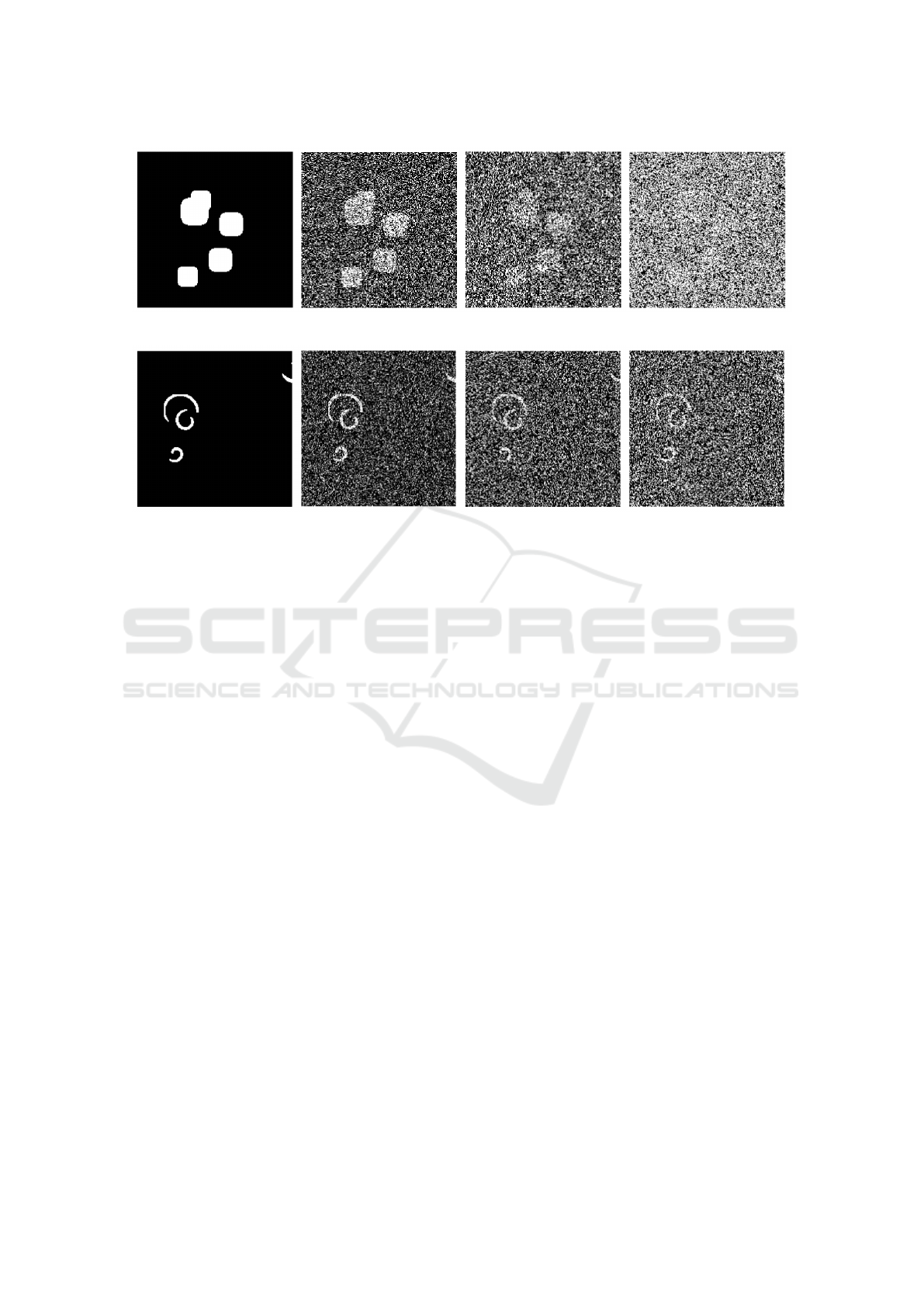
Figure 1: Zoom in for the sphere noise scenario with noise intensities η = [0, 1, 2, 3] from left to right, respectively.

Figure 2: Zoom in for the spiral noise scenario with noise intensities η = [0, 0.5, 0.75, 1] from left to right, respectively.

(LL) and luminescence variability (LV) throughout

the z dimension by additionally reducing the intensity

of each slice away from the middle of a factor ι. In de-

pendence to the experimental setting this is one likely

scenario but in different settings the LV can have also

an inverse character where the middle average inten-

sity is lower than at the borders. Since PRAQA works

in a 2D slice-speciﬁc mode, the direction of LL and

LV does not affect the results.

We compare our algorithm with BM3D (Dabov

et al., 2007), median ﬁltering (Lim, 1990), non-local

means ﬁltering (Buades et al., 2005) and wavelet de-

noising (Donoho, 1995). We parameterized BM3D

with σ = 60 without reporting benchmarks with lower

values since this conﬁguration always performed bet-

ter than others. By contrast, we parameterized me-

dian ﬁltering with different neighborhoods (5, 10 and

15 pixels) because in dependence on the input the

different parameterization exhibited different perfor-

mances. Since our algorithm directly outputs a bi-

nary image, we then used either a global thresh-

old, Otsu method (Otsu, 1979) or Niblack threshold-

ing (Niblack, 1985), for binarizing the results of the

benchmark algorithms. All algorithms implementa-

tions are based on MATLAB and we used the native

MATLAB implementations for all the competing al-

gorithms except for BM3D for which the implemen-

tation of the original paper was used (Dabov et al.,

2007).

In the following sections, we will refer to BM3D

(σ = 60) as B60, to median ﬁltering with the different

neighborhood settings as M5, M10 and M15, to non-

local means ﬁltering as NLF, to wavelet denoising as

WAV and to our algorithm as PRA.

3.1 Accuracy Benchmark

In this section we evaluate the algorithms perfor-

mance by means of Receiver Operating Char-

acteristic (ROC) curve and Precision-Recall (PR)

curve (Saito and Rehmsmeier, 2015). In these ﬁrst

tests, we did not apply intensity changes (ι = 0) and

evaluated the average performance on slices in differ-

ent noise conditions with η = (1, 2, 3) for the sphere

scenario and η = (0.5, 0.75, 1) for the spiral scenario,

respectively.

For the alternative approaches, the performance

curves were obtained by changing the global inten-

sity threshold after ﬁltering. Since PRAQA directly

returns a binarized image, the performance curve was

obtained by changing θ. To avoid the use of a trained

classiﬁer which could unevenly bias the result, we

kept only one feature of the 3 features obtained by cir-

cular SEs. In particular, we chose the largest SE for

the sphere scenario and the smallest SE for the spiral

scenario, respectively.

Table 3 and 2 report the Area Under Curve

(AUC) for both the sphere and spherical scenario, re-

spectively. Without intensity changes along the z di-

mension, BM3D performs best and in particular better

than PRAQA. Still, PRAQA performs typically bet-

ter than all the other algorithms and yields acceptable

results in all cases except in the noisiest spiral sce-

nario. The great performance of BM3D is based on

BIOIMAGING 2021 - 8th International Conference on Bioimaging

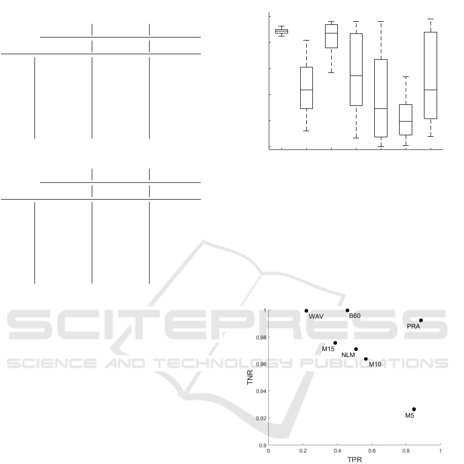
Table 2: Spiral scenario accuracy benchmark.

η = 1 η = 2 η = 3

ROC PR ROC PR ROC PR

PRA .99 .99 .99 .94 .98 .77

B60 .99 .99 .99 .96 .99 .88

M5 .99 .88 .90 .28 .80 .10

M10 .99 .98 .98 .79 .93 .45

M15 .99 .98 .99 .90 .97 .71

NLF .99 .98 .98 .78 .94 .44

WAV .99 .97 .99 .84 .97 .61

Table 3: Sphere scenario accuracy benchmark.

η = 0.5 η = 0.75 η = 1

ROC PR ROC PR ROC PR

PRA .99 .87 .99 .70 .97 .45

B60 .99 .91 .99 .80 .99 .68

M5 .99 .81 .97 .53 .94 .24

M10 .98 .55 .97 .43 .95 .28

M15 .98 .35 .97 .29 .94 .20

NLF .99 .91 .98 .60 .95 .25

WAV .97 .63 .93 .33 .88 .14

its speciﬁc focus on white Gaussian noise and its per-

formance still remains a gold standard nowadays.

3.2 Performance with LV Benchmark

Next, we investigated the performance of the algo-

rithms in a scenario with both noise and intensity

changes. We ﬁxed ι = 0.03 and η = 0.75 in the spiral

scenario and measured the performance with respect

to true positive rate (TPR) and true negative rate

(TNR). The MAD

threshold parameter θ was set to 3.

Since using just one global threshold for the binariza-

tion for the competing algorithms would be unfair, we

picked automatically a threshold for each slice by the

Otsu method and Niblack thresholding. In Figure 3,

the variability of TPR among slices for the different

algorithms is shown. We empirically assess the ro-

bustness of PRAQA with respect to intensity changes

among slices emphasized by the small TPR variance

compared to the other methods. This result further

demonstrates the great potential of PRAQA for im-

ages with high LV that is typically observed in tissue

staining.

In Figures 4 and 5, we next investigated the perfor-

mance of the algorithms by averaging TPR and TNR

slice-wise for the different threshold approaches, re-

spectively. These plots indicate that PRAQA robustly

binarizes images with high accuracy since it exhibits

high TPR and TNR while the alternative algorithms

typically are more targeted for one criterion. Thus,

PRA B60 M5 M10 M15 WAV NLM

0.2

0.4

0.6

0.8

TPR

Figure 3: TPR Boxplot slicewise.

WAV and B60 exhibited a slightly higher TNR com-

pared to PRAQA but performed signiﬁcantly worse

with respect to TPR using Otsu thresholding (Fig. 4).

For Niblack thresholding, WAV resulted in a higher

TPR than PRAQA but had the worst TNR perfor-

mance of all algorithms (Fig. 5). Hence, the tar-

geted approach of PRAQA represents a good compro-

mise for binarization that signiﬁcantly outperforms

the other algorithms.

Figure 4: Performance Scatter Plot with Otsu thresholding.

3.3 Robustness against Positive Pixel

Content

To investigate the performance of PRAQA in depen-

dence on signal (i.e. object) density, we ﬁxed the

threshold parameter θ in the binarizedMAD routine

(Section 2.1) and considered the spiral scenario with

η = [0.5,0.75] and ι = 0.03. We ﬁrst investigated the

dependency of MAD (Eq. 1) with respect to the num-

ber of objects and subsequently conﬁrmed the results

in the synthetic scenario. For this purpose, we in-

creased the number of objects by adding a multiplying

constant to the number of objects listed in Table 1.

PRAQA: Protein Relative Abundance Quantiﬁcation Algorithm for 3D Fluorescent Images

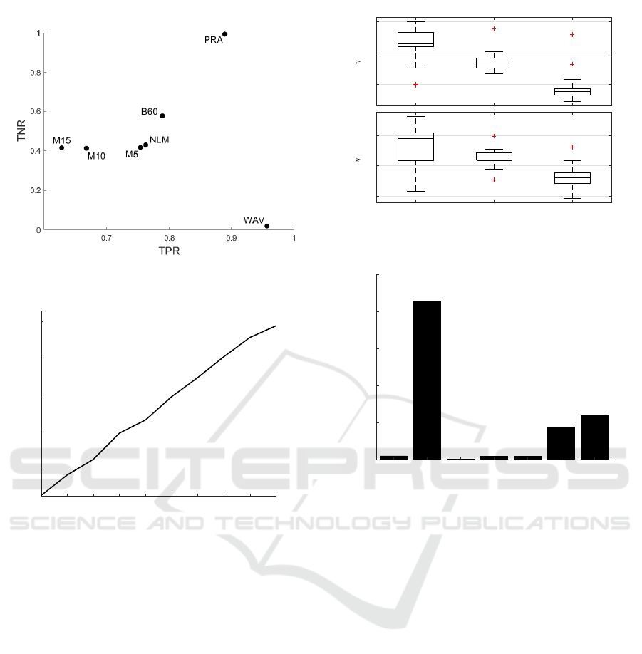
Figure 5: Performance Scatter Plot with Niblack threshold-

ing.

1 3 5 7 9 11 13 15 17 19

Object Density

1.35

1.351

1.352

1.353

1.354

MAD

Figure 6: Variation of MAD with respect to object density.

In Figure 6, we observe a linear dependency be-

tween the amount of positive signal given by the ob-

ject density and resulting MAD values. Thus, the

MAD scaling factor used to obtain MAD

as deﬁned

by Eq. 1 leads to changes in the algorithm positive

pixels detection. Figure 7 depicts the change of TPR

in a spiral scenario with a ﬁxed θ = 3 for an increase

of objects increases by 10 and 20 times and two differ-

ent noise intensities. Interestingly, we observed only a

minor loss in TPR of 0.008 for a 10 fold change in the

amount of positive signal when noise is low (η = 0.5)

and 0.025 for larger noise (η = 0.75). Even for the

higher density with a scaling factor of 20, the reduc-

tion in TPR is relatively low following the linear de-

pendency and further demonstrates the robustness of

PRAQA.

3.4 Runtime Benchmark

To investigate the applicability of the different algo-

rithms also with respect to real-world applications, we

benchmarked the time required to process 30 slices

0.97

0.98

0.99

TPR ( = 0.5)

1 10 20

0.8

0.85

0.9

TPR ( = 0.75)

Figure 7: Boxplots of TPR performance with respect to ob-

ject density (top: η = 0.5, bottom: η = 0.75).

51.9

2132.7

7.1

46.3

46.9

437.7

596.5

PRA B60 M5 M10 M15 NLF WAV

500

1000

1500

2000

2500

Runtime (s)

Figure 8: Runtime in seconds for each algorithm.

of size 2048 by 2048 pixels. The machine used

for benchmarking was equipped with two Intel Xeon

E5645 @2.40 Ghz and 96 GB RAM. Figure 8 depicts

a bar plot for each tested algorithm demonstrating

that PRAQA exhibits a great runtime performance. In

particular, PRAQA performs signiﬁcantly better com-

pared with the second accurate algorithms WAV and

BM3D (B60) with a 40 times faster performance than

BM3D. The PRAQA algorithm execution time is in-

dependent with respect to the choice of θ but directly

proportional to the number of SEs.

A GPU parallelized version of the algorithm has

also been developed. However, most of the time

needed for the processing is taken by the MAD eval-

uation, which is not a parallelizable operation when

the exact MAD values are computed. A faster solu-

tion can be obtained by losing accuracy in the mea-

surement via pixel intensity binning, which may make

PRAQA be even suitable for real time applications.

Overall, the extensive benchmarking of PRAQA has

shown that its targeted approach for 3D ﬂuoresecent

images with LV and LL outperforms alternative algo-

rithms in terms of accuracy and runtime.

BIOIMAGING 2021 - 8th International Conference on Bioimaging

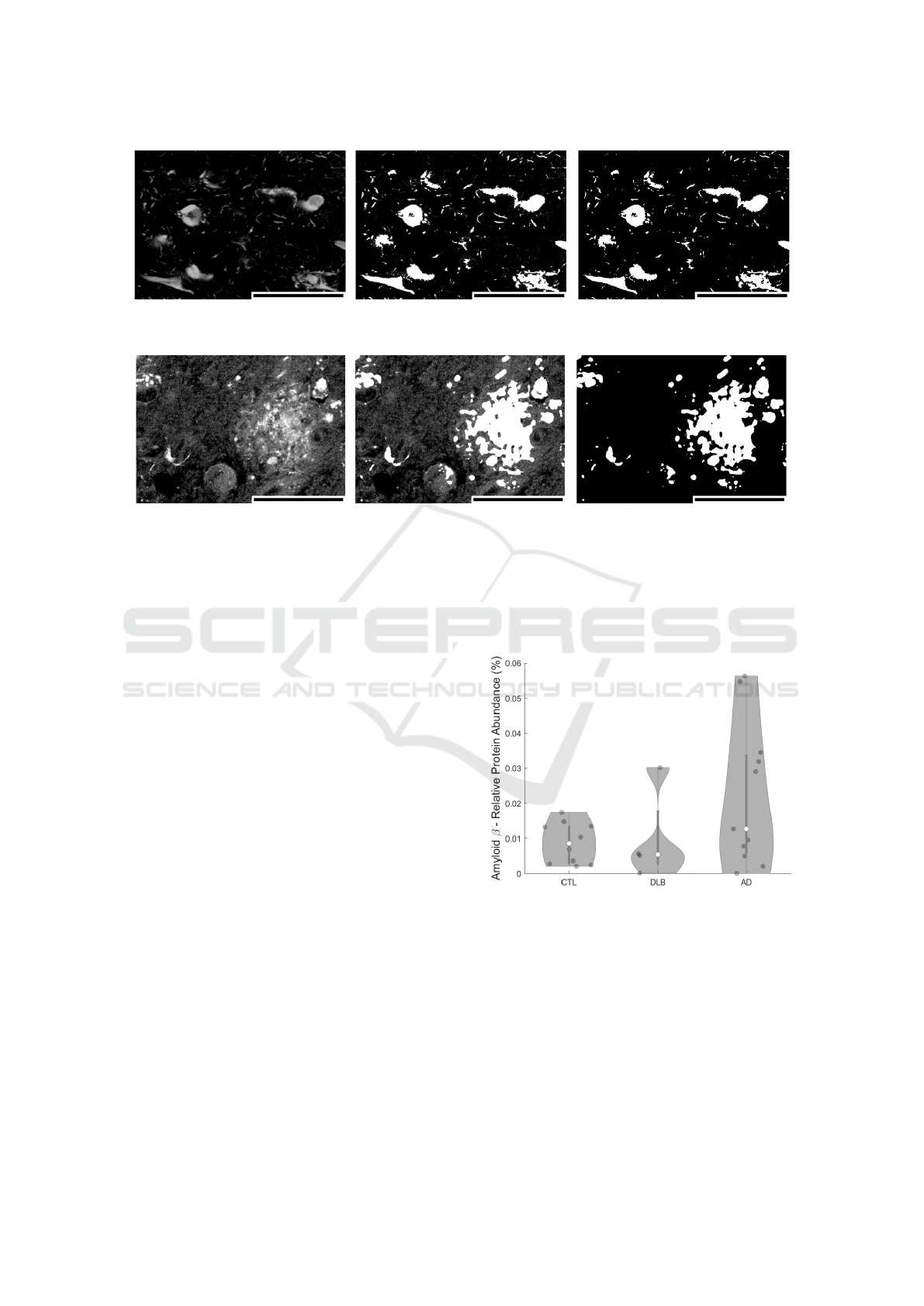
Figure 9: Hyperphosphorylated tau aggregation by AT8-staining acquisition in a region of interest. From left to right: original

acquisition, original + PRAQA overlay, PRAQA. Scale bar: 60 µm.

Figure 10: Amyloid-beta aggregation by 4G8-staining acquisition in a region of interest. From left to right: original acquisi-

tion, original + PRAQA overlay, PRAQA. Scale bar: 60 µm.

4 REAL SCENARIO

Based on the successful benchmarking of PRAQA

with the synthetic scenarios in Section 3, we next

applied PRAQA to a real world application of neu-

rodegeneration (Salamanca et al., 2019). A common

feature of different neurodegenerative diseases such

as Alzheimer’s or Parkinson’s disease is the accumu-

lation of proteins either intracellular or extracellular

(Ross and Poirier, 2004). While the function and im-

pact of these aggregates is still not fully understood,

they are essential for the diagnosis. Current biomedi-

cal research is focusing on the characteristics of these

protein aggregates and their relation to different dis-

ease stages (Dugger and Dickson, 2017). For this pur-

pose, a reliable quantiﬁcation approach of protein ag-

gregation in tissue is essential and PRAQA is exactly

targeting this need.

Here, we demonstrate the potential of PRAQA in

the context of Alzheimer’s Disease (AD) and De-

mentia with Lewy Bodies (DLB). Both conditions

share the accumulation of extracellular aggregation

of amyloid-beta 1-42 and intracellular aggregation

of hyperphosphorylated tau in the parenchyma but

with an higher burden expected in AD samples. To

characterize amyloid and tau aggregation in a cohort

of human post-mortem brain samples (Tab. 4), we

have stained our collection of samples with antibod-

ies commonly used in neuropathology to vizualize re-

spective protein/peptide aggregation (Figs. 9 and 10),

acquired 3D stacks with a confocal microscope and

performed relative protein abundance quantiﬁcation

with PRAQA (Figs. 11 and 12).

Figure 11: Amyloid peptide abundance per sample condi-

tion stained by 4G8.

4.1 Human Brain Sections Preparation

and Data Acquisition

Anonymized human brain samples were provided

by the Douglas-Bell Brain Bank (Douglas Mental

Health University Institute, Montr

eal, QC, Canada)

and all experiments were conducted in accordance

with the guidelines approved by the Ethics Board of

the Douglas-Bell Brain Bank and the Ethics Panel of

PRAQA: Protein Relative Abundance Quantiﬁcation Algorithm for 3D Fluorescent Images

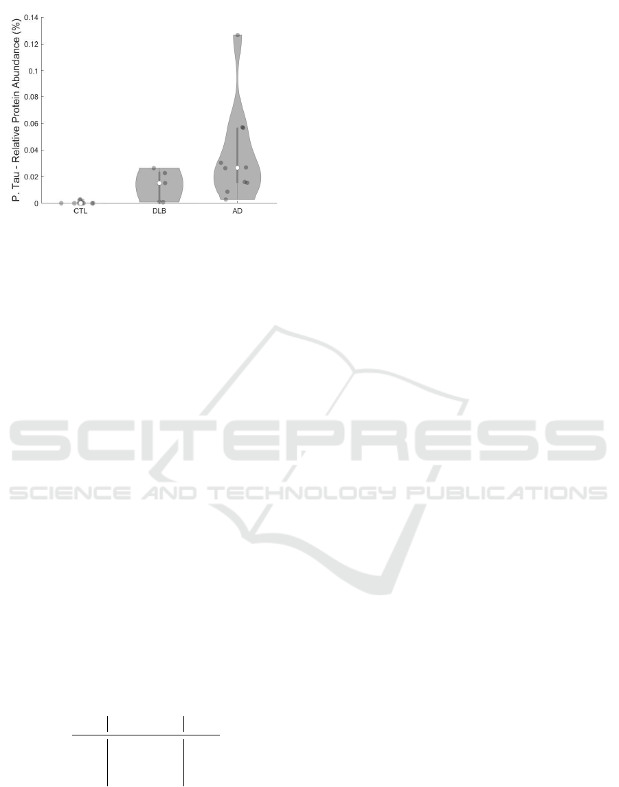
Figure 12: P-tau protein abundance per sample condition

stained by AT8.

University of Luxembourg. For this study, cases of

neuropathologically conﬁrmed AD and DLB, as well

as from age-matched controls (CTLs) were selected.

Immunohistochemistry protocol was performed as

previously described (Bouvier et al., 2016) (Ques-

seveur et al., 2019). Brieﬂy, sections were im-

munostained with the primary antibody Mouse anti-

4G8 (amyloid-beta) (Biolegend [800712]) or Mouse

anti-AT8 (hyperphosphorylated tau) (Thermoﬁsher

[MN1020]). Afterwards, sections were incubated

with secondary antibodies Donkey anti-Mouse Alexa

Fluor 488 (4G8) or 647 (AT8) (Jackson ImmunoRe-

search Laboratories, West Grove, PA and Invitrogen,

Molecular Probes, Eugene, OR) and mounted. Flu-

orescent 3D confocal tile scans were captured and

stitched on a confocal Zeiss Laser Scanning Micro-

scope710 with a 20x air objective. Tile scans were

acquired to cover a larger area of the CA1 subﬁeld of

the hippocampus. Identical image acquisition param-

eters were respectively used for each of the staining

on all samples.

4.2 Dataset and Processing

Table 4 reports the number of acquisitions processed

in this study grouped by condition.

Table 4: Number of samples per condition and marker.

Amyloid β Tau

CTL 11 12

AD 13 12

DLB 4 5

To compute the positive pixel sum coming from

the binarized image processed by PRAQA, we used

a parameterization of θ = 5 for all images except for

three CTL samples with 4G8 staining for which we

used θ = (8, 8, 10) to counteract a higher presence of

noise. Each sample had on average 25 slices separated

by 1 µm in the third dimension. For some samples, be-

ginning and/or ending slices had to be removed due to

tile-related artifacts occurred during the microscope

acquisition. For ﬁnal analysis, the positive pixel sum

was normalized to the 3D image size.

4.3 Results

Figures 9 and 10 show a region of interest (ROI) of

AT8 and 4G8 stained structures in post-mortem AD

brains. The ROI is the CA1 subﬁeld of the hip-

pocampus, a brain region involved in memory con-

solidation and retrieval and known to be severely af-

fected by AD. AT8 staining reveals intraneuronal ﬁb-

rillar structures called neuroﬁbrillary tangles(Goedert

et al., 1995) and 4G8 staining shows accumulations

of the amyloid-beta peptide in intracellular inclusions

and extracellular plaques (Hunter and Brayne, 2017).

These protein accumulations are considered typical

neuropathological hallmarks of Alzheimer’s Disease

and are clinically used to assess disease staging. All

structural details of both stainings are preserved af-

ter PRAQA processing (Figure 9) and the presence

of noise is counteracted in the example of the 4G8

stained sample (Figure 10).

The comparison between the original acquisitions

and the by PRAQA binarized images demonstrates

that PRAQA is capable to segment the qualitatively

different protein aggregations successfully as vali-

dated by visually inspection of the overlay of the

original images and the PRAQA output by a neu-

ropathology expert. For the hyperphosphorylated tau

staining, the original image does not exhibit strong

background signal and PRAQA resolved also subtle

structures (Fig. 9). The original amyloid-beta stain-

ing has a stronger background signal and less well-

deﬁned structures. In this scenario, PRAQA did not

resolve all potential substructures but successfully

classiﬁed positive pixels that represent the amyloid-

beta plaques (Fig. 10).

As a demonstration how PRAQA can be used for

disease classiﬁcation, Figures 11 and 12 show the rel-

ative protein abundance in dependence on the sam-

ple condition. The analysis of amyloid-beta pep-

tide abundance within the CA1 hippocampal sub-

ﬁeld shows in agreement with literature an enriche-

ment overall of amyloid-beta level in AD samples

(Marti Colom-Cadena, 2013). Interestingly, a lower

and residual amyloid-beta presence is also revealed

in age-matched controls as well as in samples from

patients with DLB. The relative abundance is here

comparable to AD samples with low Amyloid bur-

den (Marti Colom-Cadena, 2013). This ﬁnding may

indicate a general age-dependent increase of amyloid-

BIOIMAGING 2021 - 8th International Conference on Bioimaging

beta aggregation even in cognitively healthy controls

which is also coherent with previous ﬁndings (Ro-

drigue, 2012).

The comparison of hyperphosphorylated tau ag-

gregation among samples exhibits an even stronger

disease dependence (Fig. 12). While CTL samples

were consistently negative for tau aggregation, AD

samples exhibited a very strong enrichment to up of

0.13%. Strikingly, some DLB samples also showed

considerable amounts of phospho-tau proteins com-

pared to the age-matched control samples with lev-

els similar to AD condition (Marti Colom-Cadena,

2013).

Overall, this ﬁrst application of PRAQA to hu-

man brain samples demonstrated that the targeted

approach allows for quantiﬁcation of protein aggre-

gation within heterogeneous tissue. Furthermore,

PRAQA analysis of amyloid-beta and hyperphospho-

rylated tau distribution in CA1 subregions of AD and

DLB cases conﬁrms that the two conditions share

common mechanisms of protein aggregation and may

represent a more continuous spectrum of cellular

pathologies than typically anticipated.

5 CONCLUSIONS

Protein function is essential for cellular and tissue

homeostasis and impairments are linked to diverse

diseases. Here, we introduced PRAQA as an efﬁ-

cient tool to quantify relative protein abundance and

localization in complex tissues from 3D ﬂuorescent

images. For this purpose, PRAQA speciﬁcally targets

luminescence variability caused by optical constraints

along the z dimension and by inter-sample variability

by applying an Median Absolute Deviation approach

for each 2D (x-y) plane of the image (Section 2).

Extensive benchmarking of PRAQA against alter-

native algorithms for synthetic scenarios has demon-

strated that the targeted approach allows for accu-

rate, robust and efﬁcient quantifcation of relative

protein abundance in cases where noise and inten-

sity changes play an important role in the measure-

ment (Section 3). In particular, we have shown

that PRAQA performs well when dealing with im-

ages compromised by intensity changes (either intra-

acquisition or inter-acquisition) and is also resilient

up to a considerable amount of noise. The key ad-

vantages of this algorithm are its simple parameteri-

zation (1-parameter), computational efﬁciency and di-

rect applicability that does not require any preprocess-

ing. These features prevent typical biases of alterna-

tive approaches based on versatile parameters which

may compromise measurements and thus the results.

However, in cases of extreme noise, dedicated multi-

parametric pipelines might be used to deal with these

peculiar situations but care has to be taken for sample

comparison.

Finally, we have used PRAQA for a real applica-

tion in neurodegeneration and quantiﬁed protein ag-

gregation in human brain samples (Section 4). In this

application, we quantiﬁed amyloid-beta and hyper-

phosphorylated tau protein aggregation in immunos-

tained brain samples of AD, DLB and control sub-

jects where PRAQA was able to segment reliably the

qualitatively different structures. The ﬁrst compari-

son of protein aggregation between the disease condi-

tions substantiates the essential role of amyloid-beta

plaques in AD but also indicates some shared proper-

ties of protein aggregation in neurodegenerative dis-

eases.

Overall, the targeted approach of PRAQA repre-

sents an efﬁcient and easy-to-use tool to investigate

spatially resolved protein abundance in health and

disease conditions.

5.1 Future Work

We plan to extend the algorithm by an additional mod-

ule to estimate an optimal range for the threshold pa-

rameter θ. This automation may be achieved by sta-

tistically inferring when false positive pixels start to

appear in a salt and pepper manner throughout the

acquisition by progressively lowering θ. Furthermore,

we will test PRAQA with other staining markers lead-

ing to different structures and potentially adapted SEs

for ad-hoc situations (e.g. ﬁlaments or branches) also

in the context of the neurodegenerative samples. In

this respect, PRAQA will be also a valuable extension

to combine morphological characterizations (Sala-

manca et al., 2019) with protein abundances for in-

vestigations of multicellular mechanisms in neurode-

generation.

CONFLICT OF INTEREST

The authors declare no competing ﬁnancial interests.

ACKNOWLEDGEMENTS

The authors thank the Douglas-Bell Brain Bank

for providing human brain samples, the Bioimag-

ing Facility of the Luxembourg Centre for Sys-

tems Biomedicine (LCSB) for support of microscopy,

the Reproducible Research Results (R3) team of

the LCSB for promoting reproducible research, R.

PRAQA: Protein Relative Abundance Quantiﬁcation Algorithm for 3D Fluorescent Images

Sassi and E. Casiraghi for fruitful discussions.

C.A. and S.F. were supported by the PRIDE pro-

gram of the Luxembourg National Research Found

through the grants PRIDE17/12252781/DRIVEN and

PRIDE17/12244779/PARK-QC, respectively. This

work was further supported by the Luxembourgish

Espoir-en-T

ete Rotary Club award, the Auguste et Si-

mone Pr

evot foundation, and the Agaajani family do-

nation for Alzheimer’s Disease research.

REFERENCES

Alberts, B. (2017). Molecular Biology of the Cell. W.W.

Norton.

Belthangady, C. and Royer, L. (2018). Applications,

promises, and pitfalls of deep learning for ﬂuores-

cence image reconstruction.

Bouvier, D. S., Jones, E. V., Quesseveur, G., Davoli, M. A.,

A Ferreira, T., Quirion, R., Mechawar, N., and Murai,

K. K. (2016). High Resolution Dissection of Reactive

Glial Nets in Alzheimer’s Disease. Sci Rep, 6:24544.

Buades, A., Coll, B., and Morel, J. . (2005). A non-local al-

gorithm for image denoising. In 2005 IEEE Computer

Society Conference on Computer Vision and Pattern

Recognition (CVPR’05), volume 2, pages 60–65 vol.

Chung, K., Wallace, J., Kim, S.-Y., Kalyanasundaram, S.,

Andalman, A., Davidson, T., Mirzabekov, J., Zalo-

cusky, K., Mattis, J., Denisin, A., Pak, S., Bernstein,

H., Ramakrishnan, C., Grosenick, L., Gradinaru, V.,

and Deisseroth, K. (2013). Structural and molecu-

lar interrogation of intact biological systems. Nature,

497.

Dabov, K. ., Foi, A. ., Katkovnik, V. ., and Egiazarian, K. .

(2007). Image Denoising by Sparse 3-D Transform-

Domain Collaborative Filtering. IEEE Transactions

on Image Processing, 16(8):2080–2095.

Donoho, D. L. (1995). De-noising by soft-thresholding.

IEEE Transactions on Information Theory,

41(3):613–627.

Dugger, B. N. and Dickson, D. W. (2017). Pathology of

neurodegenerative diseases. Cold Spring Harbor per-

spectives in biology, 9(7):a028035. 28062563[pmid].

Goedert, M., Jakes, R., and Vanmechelen, E. (1995). Mon-

oclonal antibody at8 recognises tau protein phospho-

rylated at both serine 202 and threonine 205. Neuro-

science Letters, 189(3):167 – 170.

Hunter, S. and Brayne, C. (2017). Do anti-amyloid beta

protein antibody cross reactivities confound alzheimer

disease research? Journal of negative results in

biomedicine, 16(1):1–1. 28126004[pmid].

Im, K., Mareninov, S., Diaz, M. F. P., and Yong, W. H.

(2019). An Introduction to Performing Immunoﬂuo-

rescence Staining. Methods Mol Biol, 1897:299–311.

Komin, N. and Skupin, A. (2017). How to address cellular

heterogeneity by distribution biology. Current Opin-

ion in Systems Biology, 3:154–160.

Leys, C., Ley, C., Klein, O., Bernard, P., and Licata, L.

(2013). Detecting outliers: Do not use standard devi-

ation around the mean, use absolute deviation around

the median. Journal of Experimental Social Psychol-

ogy, 49(4):764 – 766.

Lim, J. S. (1990). Two-Dimensional Signal and Image Pro-

cessing. Prentice-Hall, Inc., USA.

Marti Colom-Cadena, E. G. (2013). Conﬂuence of a-

synuclein, tau, and b-amyloid pathologies in demen-

tia with Lewy bodies. J. Neuropathol. Exp. Neurol.,

72(12):1203–1212.

Niblack, W. (1985). An Introduction to Digital Image Pro-

cessing. Strandberg Publishing Company, DNK.

Otsu, N. (1979). A threshold selection method from gray-

level histograms. IEEE Transactions on Systems,

Man, and Cybernetics, 9(1):62–66.

Quesseveur, G., Fouquier d’Herouel, A., Murai, K. K., and

Bouvier, D. S. (2019). A Specialized Method to Re-

solve Fine 3D Features of Astrocytes in Nonhuman

Primate (Marmoset, Callithrix jacchus) and Human

Fixed Brain Samples. Methods Mol. Biol., 1938:85–

95.

Rodrigue, K. M. (2012). β-amyloid burden in healthy ag-

ing: regional distribution and cognitive consequences.

Neurology, 78(6):387–395. 22302550[pmid].

Ross, C. A. and Poirier, M. A. (2004). Protein aggrega-

tion and neurodegenerative disease. Nature Medicine,

10(7):S10–S17.

Saito, T. and Rehmsmeier, M. (2015). The precision-recall

plot is more informative than the roc plot when evalu-

ating binary classiﬁers on imbalanced datasets. PLOS

ONE, 10(3):1–21.

Salamanca, L., Mechawar, N., Murai, K. K., Balling, R.,

Bouvier, D. S., and Skupin, A. (2019). Mic-mac: An

automated pipeline for high-throughput characteriza-

tion and classiﬁcation of three-dimensional microglia

morphologies in mouse and human postmortem brain

samples. Glia.

Varghese, F., Bukhari, A. B., Malhotra, R., and De, A.

(2014). Ihc proﬁler: An open source plugin for the

quantitative evaluation and automated scoring of im-

munohistochemistry images of human tissue samples.

PLOS ONE, 9(5):1–11.

BIOIMAGING 2021 - 8th International Conference on Bioimaging