
Empirical Evaluation on Utilizing CNN-features for Seismic Patch
Classification
Chun-Xia Zhang
1 a
, Xiao-Li Wei
1 b
and Sang-Woon Kim
2 c
1
School of Mathematics and Statistics, Xi’an Jiaotong University, Xi’an, 710049, China
2
Department of Computer Engineering, Myongji University, Yongin, 17058, South Korea
Keywords:
Seismic Patch Classification, Feature Extraction, CNN-features, Transfer Learning.
Abstract:
This paper empirically evaluates two kinds of features, which are extracted respectively with neural networks
and traditional statistical methods, to improve the performance of seismic patch image classification. The
convolutional neural networks (CNNs) are now the state-of-the-art approach for a lot of applications in var-
ious fields, including computer vision and pattern recognition. In relation to feature extraction, it turns out
that generic feature descriptors extracted from CNNs, named CNN-features, are very powerful. It is also well
known that combining CNN-features with traditional (non)linear classifiers improves classification perfor-
mance. In this paper, the above classification scheme was applied to seismic patch classification application.
CNN-features were acquired first and then used to learn SVMs. Experiments using synthetic and real-world
seismic patch data demonstrated some improvement in classification performance, as expected. To find out
why the classification performance improved when using CNN-features, data complexities of the traditional
feature extraction techniques like PCA and the CNN-features were measured and compared. From this com-
parison, we confirmed that the discriminative power of the CNN-features is the strongest. In particular, the
use of transfer learning techniques to obtain CNN’s architectures to extract the CNN-features greatly reduced
the extraction time without sacrificing the discriminative power of the extracted features.
1 INTRODUCTION
Recently, seismic wave fault detection using deep
learning techniques has been actively studied (Cunha,
A. et al., 2020), (Di, H. et al., 2018), (Hung, L. et al.,
2017), (Pochet, A. et al., 2019), (Wang, Z. et al.,
2018). In this approach, seismic images are first di-
vided into patches of a certain size. The fault detec-
tion problem then becomes a two-class classification
problem that classifies fault and non-fault (normal)
patches. The fault detection problem can be solved
by identifying the location of patches classified as ab-
normal patches in the fault line. This paper focuses
on the classification of patch data. First, feature vec-
tors are extracted from seismic patch data and then
classified as fault and non-fault patches using existing
classifiers to find fault lines.
Convolutional neural networks (CNNs) are now
state-of-the-art approach for a lot of applications.
a
https://orcid.org/0000-0001-9639-4507
b
https://orcid.org/0000-0003-1383-8040
c
https://orcid.org/0000-0002-3172-8462
Based on their good performance, CNNs have re-
cently been used to detect seismic faults (Pochet, A.
et al., 2019). However, two constraints can be found
in this approach: one is the need to provide a huge
number of interpreted data (e.g., fault and nonfault
patches); the other is a significant amount of time re-
quired to process them. To address the first, a syn-
thetic data set having simple fault geometries has been
built. Therefore, the input to the CNN is the seismic
amplitude only. That is, the approach does not require
the calculation of the other seismic attributes, but the
second constraint remains without any solution.
As is commonly known, CNN takes a tremendous
amount of time to learn when allowing “sufficient”
training data. Recently, it has been observed that
the convolutional (C) and fully-connected (FC) lay-
ers take most of the time to run (Donahue, J. et al.,
2014). In particular, since the latter is responsible
for multiplication of large-scale matrices, it consumes
most of the computation time up to 60%. From the
above review results and the findings in (Alshazly,
H. et al., 2019), (Athiwaratkun, B. and Kang, K.,
2015), (Donahue, J. et al., 2014), (Girshick, R. et al.,
166
Zhang, C., Wei, X. and Kim, S.
Empirical Evaluation on Utilizing CNN-features for Seismic Patch Classification.
DOI: 10.5220/0010185701660173
In Proceedings of the 10th International Conference on Pattern Recognition Applications and Methods (ICPRAM 2021), pages 166-173
ISBN: 978-989-758-486-2
Copyright
c
2021 by SCITEPRESS – Science and Technology Publications, Lda. All rights reserved

2014), (Razavian, L. et al., 2014), and (Weimer, D.
et al., 2016), we may consider replacing the FC lay-
ers responsible for classifying seismic patch data us-
ing CNN with existing classifiers such as support vec-
tor machines (SVMs). The role of the C layer in this
framework is the same as that of PCA (principal com-
ponent analysis), for example.
The use of SVMs instead of FC layers is known
to improve classification accuracy (Lin, T.-Y. et al.,
2015), but no analysis has been made on why. Rather
than embarking on a general analysis, in this paper we
will consider comparative studies that will be taken
as the basis for the above improvements. In addition,
measures of data complexity can be used to estimate
the difficulty in separating the sample points into their
expected classes. Especially, it has been reported that
the measurements are performed to figure out a va-
riety of characteristics related to data classification
(Lorena, A. C. et al., 2018). From this point of view,
to derive an intuitive comparison and to answer the
above question, we will consider the measurements.
In this paper we use CNN-features in seismic
patch classification. This feature allows CNN to avoid
learning time problems without compromising perfor-
mance. We also analyze data complexity to compare
the discriminating power of the features. The fol-
lowing sections in turn describe the relevant studies,
methods and results of experiments, conclusions, etc.
2 RELATED WORK
In this section we first briefly review some of the latest
results related to the design and performance evalua-
tion of the classifiers using the features extracted from
CNNs.
2.1 CNN-features
CNN-features consist of the values taken from the
activation units of the first FC layer of the CNN ar-
chitecture (Athiwaratkun, B. and Kang, K., 2015).
Various studies have been conducted using CNN-
extracted features in many applications. First, in
(Oquab, M. et al., 2014), it is evaluated whether CNN
weights obtained from large-scale source tasks could
be transferred to a target task with a limited amount of
training material. Along with this study, many studies
on related to the extraction and utilization of CNN-
features have been conducted (Razavian, L. et al.,
2014), (Donahue, J. et al., 2014), (Zeiler, M. D. and
Fergus, R., 2014), (Girshick, R. et al., 2014).
Then, in (Hertel, L. et al., 2015), it was re-
ported again that reusing a previously trained CNN
as generic feature extractors leads to a state-of-the-art
result, meaning that CNNs are able to learn generic
feature extractors that can be used for different tasks.
Thus, some studies have recently been reported in the
industry on the techniques of extracting and then clas-
sifying feature vectors with this approach (Weimer, D.
et al., 2016), (Alshazly, H. et al., 2019).
In addition, in (Alshazly, H. et al., 2019), seven
best-performing hand-crafted descriptors were com-
pared with four CNN-based models using variants of
AlexNet (Krizhevsky, A. et al., 2012). Experiments
on three data sets reported that CNN-based models
were very superior to other models. However, it was
also pointed out that, to extract meaningful features
from raw data, the approach requires huge amounts
of training data. In case the generation of the data is
expensive, it might not be appropriate, as in (Sun, C.
et al., 2017).
2.2 Data Complexity
An attempt to identify the relationship between the
data and the classifier that classifies it was specifically
initiated in (Ho, T. K. and Basu, M., 2002). Since
then, it has been studied a lot. A few of them, but
not all, can be found in: (Sotoca, J. M. et al., 2006),
(Cano, J.-R., 2013), (Lorena, A. C. et al., 2018).
Measurements of data complexity can be divided
into three groups: (i) overlapping measurements of in-
dividual feature values, e.g. Fisher’s discriminant ra-
tio (F1), directional-vector Fisher’s discriminant ratio
(F1v or simply Fv), volume of overlap region (F2),
and maximum individual feature efficiency (F3), (ii)
measuring separability of grade, e.g. non-parametric
separability of classes (N2), distance of erroneous in-
stances to a linear classifier (L1) or its training error
rate (L2), and (iii) neighborhood measures, e.g. vol-
ume of local neighborhood (D2)
1
.
On the other hand, the data complexity measure-
ments mentioned above have been used for various
applications such as meta-analysis of classifiers, pro-
totype selection, and feature selection. In addition,
another application that enables the proper use of
complexity measurements in deep learning is an ap-
plication that analyzes and organizes the capabilities
of a number of learning algorithms by application
area. In this paper we are going to use the data com-
plexities to explain why using the CNN-features im-
proves classification performance.
1
A detailed description of each of these parameters is
omitted here, but can be found in the literature.
Empirical Evaluation on Utilizing CNN-features for Seismic Patch Classification
167

3 METHODS AND DATA
This section first introduces the classification meth-
ods associated with current empirical research, then
provides the structure of seismic wave image data de-
veloped in this paper.
3.1 Classification Methods
The classification of the seismic patch data (as de-
scribed in Section 3.2) in this paper is carried out
by a method (named HYB) that hybridizes the exist-
ing linear (nonlinear) classifier (e.g., SVM) and the
convolution neural network. HYB is a classification
framework in which feature extraction is performed
on CNN from input seismic patches and then SVM is
trained using the extracted features. In particular, a
pretrained CNN model is used for initialization when
extracting CNN-feature vectors.
In HYB, feature vectors are obtained in the CNN
architecture (as described in Section 4.1) as follows:
this is an mid-level representation just before the in-
put image passes through the C layers that make up
the CNN and then passes it to the FC layers. There-
fore, the dimension of the feature vectors is equal to
the number of neurons that make up the first FC layer.
As a result, the CNN-specific dimensions can be op-
timized by determining the number of FC input neu-
rons appropriate for a given application.
To extract CNN-features as described above, the
CNN’s weights that make up the C layers should be
fixed in advance. To this end, transfer learning tech-
niques can be used. In transfer learning, the cardinal-
ity of the dataset of the target task is less than that of
the training dataset of the source task. Therefore, the
CNN-feature extraction method can avoid the com-
mon problem of CNN needing a large amount of data
for learning. In addition, CNN learning in the transfer
learning mode is made up of fine-tuning. Therefore,
a small number of epochs can significantly reduce the
learning time.
3.2 Seismic Data
Fig. 1 presents an example of a synthetic seismic wave
image (left) and a fault line (right) to be extracted
from it. The data set of the synthetic seismic wave im-
ages (501 × 501 pixels), reproduced through the open
source code IPF
2
, is an artificial implementation of
sequential rock deformation over time.
A total of 500 seismic images have been prepared,
and each of them contains one fault line with differ-
ent slopes and positions. The corresponding fault po-
2
https://github.com/dhale/ipf
Figure 1: Plots presenting a synthetic seismic image (left)
and a fault line (right). Blocks marked in red and blue indi-
cate fault and non-fault patches respectively.
sition in each image was indicated in white by gener-
ating binary masks, referring to the seismic amplitude
information.
From the data set composed of image pairs shown
in Fig. 1 (where, the two images on the left and right
side include seismic waves and fault lines respec-
tively), the fault and non-fault patches were extracted.
One patch is a (45 × 45)-dimensional matrix with one
candidate pixel in the center and 2024 pixels adja-
cent to it
3
. This patch can be classified as a fault
patch or non-fault patch according to the following
rule: if the candidate pixel is a pixel forming a fault
line, then it becomes a fault patch; otherwise it be-
comes a non-fault patch. For example, referring to the
fault line matrix shown in Fig. 1 (right), all possible
fault patches were first extracted and then the same
number of non-fault patches were randomly extracted
from the seismic wave image shown in Fig. 1 (left).
4 EXPERIMENT
In this section we present the evaluation results on
experimental datasets and comparisons to the related
methods. For kernel- PCA (kPCA) using ‘gaussian’
kernel (Wang, Q., 2012)
4
and discriminative Auto-
Encoder (AE) (Gogna, A. and Majumdar, A., 2019)
5
,
the original implementations provided by the authors
were used without change. CNN was implemented
in the simplest structure to perform basic functions
6
.
Then, SVM was realized from LIBSVM
7
.
3
This is known to be the smallest patch size that pro-
vides satisfactory results (Pochet, A. et al., 2019).
4
https://www.mathworks.com/matlabcentral/file-
exchange/39715-kernel-pca-and-pre-image-reconstruction
5
https://www.mathworks.com/matlabcentral/file-
exchange/57347-autoencoders
6
https://github.com/rasmusbergpalm/DeepLearnToolbox
7
https://www.csie.ntu.edu.tw/
∼
cjlin/libsvm/
ICPRAM 2021 - 10th International Conference on Pattern Recognition Applications and Methods
168

Table 1: The CNN architecture implemented.
descriptions IN OUT outputmaps kernelsize
convolution 45 × 45 40 × 40 4 6
subsampling 40 × 40 20 × 20
convolution 20 × 20 16 × 16 8 5
subsampling 16 × 16 8 × 8
fully connected 8 × 8 2 × 1
4.1 Experimental Data
The CNN-feature extractor was tested and compared
with traditional ones such as PCA, kPCA, and AE.
Here PCA was chosen as one of the best known linear
extractors, and kPCA as one of the nonlinear versions.
In addition, AE was included as one of the feature ex-
tractors that could be implemented in a network based
manner. Experiments were performed using seismic
patch data, named Train1 (Train2 and Test1).
From the total 500 seismic wave images, three
patch sets of ‘Test1’, ‘Train1’, and ‘Train2’ were con-
structed as follows: Test1 is a set of 76, 038 patches
extracted from the first 100 images; Train1 is a set
of 74, 046 patches extracted from 100 images from
101 to 200; and Train2 is a set of 290, 074 patches
extracted from 400 seismic images from 101 to 500.
Train1 and Test1 were used to extract and evaluate
CNN-features, and Train2 was used to generate pre-
trained models needed to extract the CNN-features.
In all experiments carried out in subsequent sec-
tions, the same training and testing process were car-
ried out. First, the features of the training data were
first extracted according to a given feature extractor,
then the features of the test data was extracted by the
same process. One SVM was learned using features
extracted from the training data and the features of the
test data were used to evaluate this SVM.
4.2 The CNN Architecture
Table 1 presents the architecture of the CNN imple-
mented in this paper. This is a structure consisting of
two C’s and subsampling layers and one FC layer, one
of the smallest scale needed for the evaluation exper-
iments we are trying to realize.
In Table 1, the last component at the bottom of
the CNN is a set of FC layers, and the number of in-
put neurons of this component is defined as the num-
ber of weights output from the previous layer. The
CNN-features we are trying to extract consist of these
input neurons that connect directly to FC. Therefore,
the dimension of the feature vector can be determined
by adjusting the number of these neurons. However,
in order to find any new feature dimension, the cor-
responding structure should be retrained. Therefore,
we first got CNN-features from CNN and then applied
PCA to this vector set to reduce the dimension to the
target dimension.
Finally, this paper deals with the 2-class problem
of classifying the image patches as normal and abnor-
mal. Therefore, it is necessary to adjust the number
of neuron units in the output layer when expanding to
multi-class problems. In addition, a softmax function
is required to obtain normalized probabilities for each
class.
The CNN shown in the table was properly learned
and evaluated using the experimental data. To do this,
various parameters, including learning rate (α), mo-
mentum (µ), batch-size (γ), and number of epochs (η),
need to be set, and we experimentally set these values
as follows: α = 1, µ = 0.5, γ = 10, and η = 100.
4.3 Experiment #1: Synthetic Data
To confirm that the use of CNN-features actually
improves classification performance, we first exper-
imented with the synthetic seismic data.
4.3.1 Comparison of Classification Accuracy
Prior to presenting the classification accuracy, the task
of using data to select optimal or near-optimal param-
eters for the experiment was considered. To achieve
the best classification accuracy, we first need to se-
lect an optimized dimension value that is neither too
large nor too small. A simple preliminary experiment
was conducted in this paper to select dimensions op-
timized for the space of CNN-features. Specifically,
the experiment showed that the highest classification
accuracy was achieved when the dimension of the fea-
ture subspace was 256. Then the number of epochs
was optimized by referring to the learning curve to
prevent overfitting.
In addition, for more successful extraction, two
types of CNN-features, CNN1- and CNN2-features,
were extracted from Train1 in different ways and
compared. The CNN1-features were extracted from
randomly initialized architectures, but the CNN2-
features were extracted using pretrained models.
From the comparison of the two classification accu-
racy rates obtained with the CNN1- and the CNN2-
features, the latter was superior to the former. This
means that using pretrained CNN models leads to an
improved performance in classification. Based on this
observation, we used the CNN2-features as CNN-
features in the following experiments. At this time,
the pretrained CNN model was prepared using Train2
(# epochs is 300). Then, using Train1 (# epochs
is 200), we fine-tuned a CNN model and extracted
CNN-features from it.
Empirical Evaluation on Utilizing CNN-features for Seismic Patch Classification
169

In general, however, there is no optimal feature ex-
tractor for all classifiers, and vice versa. Thus, various
classifiers were first applied to verify the performance
of CNN-based extractors. Table 2 shows a numerical
comparison of classification accuracy measured by
NNs (nearest neighbor rules) and SVMs
8
. Here the
process of evaluating classification performance by
randomly selecting a subset of 20, 000 (and 15, 000)
from Train1 (and Test1) was repeated ten times and
the results obtained were averaged. In each iteration,
a pretrained model fine-tuned by one subset of Train1
was jointly used.
From the comparison shown in Table 2, it can be
re-observed that the use of the CNN-based extrac-
tor in conjunction with existing classifiers can signif-
icantly improve classification accuracy compared to
other extractors included in the comparison. It is note-
worthy that the CNN-based extractor uses not only
training data but also pretrained CNN models that
could not be used for other extractions. Under this
condition, direct comparison of the four feature ex-
tractors may not be fair. However, from the perspec-
tive of machine learning, such as transfer learning,
the results of this experiment are shown to suggest
one possibility related to the new feature extractor.
From this consideration, the performance improve-
ments observed in the last column of the table may
have resulted from the discriminating ability of the
pretrained models.
In addition to using the accuracy of numerical
metrics, classification performance can also be com-
pared using ROC (receiver operating characteristic)
curves. From the ROC curves obtained, it was
revealed that the CNN-features have generated the
curve closest to the upper left corner and the highest
AUC (area under the curve) value.
4.3.2 Comparison of Data Complexities
To highlight why the use of the CNN-features im-
proves classification performance, complexity mea-
sures were also measured and compared. Fig. 2 com-
pares the complexity measures obtained by applying
the four extractors to two data, Train1 and CIFAR-100
(Krizhevsky, A., 2009). Here the latter was used in
reference experiments for comparison. The original
CIFAR data were converted into a 45 × 45 grayscale
set consisting of 20 classes for testing under the same
conditions. Then, only two classes of 5, 000 (and
1, 000) samples were selected “randomly” as training
8
Each of these two classifiers was chosen as one of the
easiest to learn and the most widely used classifiers. There-
fore, thorough evaluation using other classifiers such as ad-
abust and decision tree is a future challenge.
(and test) data.
In Fig. 2, it can be observed that the relative mag-
nitude of the measured complexity values from the
feature vectors extracted in four ways is mostly very
similar. For easy observation, consider together the
accuracy rate of Table 2 and the data complexity of
Fig. 2. Compared to the accuracy of PCA and CNN-
features in Table 2, CNN-based is superior to PCA.
In Fig. 2, when comparing the F1 complexity values
for these two extractors, the CNN-based bar height is
higher than that of the PCA. However, the comparison
of Fv, D2, and L2 complexity is the opposite. Specif-
ically, the fact that the CNN-based accuracy rate in
Table 2 is greater than that of PCA is consistent with
the fact that the CNN-based F1 bar in Fig. 2 is higher
than that of PCA. However, the comparison of Fv val-
ues is the opposite. The Fv value is small when the
accuracy rate is large. As already reported in the rele-
vant literature, the increasing value of F1 reduces the
overlapping feature space and thus allows better sep-
aration of the feature space of the two classes. Unlike
F1, the smaller the value measured in Fv, the sim-
pler the classification problem. Similar comparative
analyses can be applied for the remaining other com-
plexity metrics.
In Fig. 2, however, F2 shows different character-
istics for CIFAR-100 and Train1. In general the larger
the F2 value, the greater the overlap between classes
and, therefore, the more difficult the classification is.
In addition, if there is at least one non-overlapping
feature, the result of the calculation expression is zero
(Lorena, A. C. et al., 2018). Furthermore, this mea-
sure differs in sensitivity from classification accuracy
depending on the type of classifier and does not pro-
duce reasonable information for use in the case of
SVM classifiers (Cano, J.-R., 2013).
From the observations made above, the CNN-
based extractor can be argued to be a good feature
extractor comparable to the AE-based as well as the
PCA (kPCA). In particular, this extractor can be ap-
plied to applications where existing extractors do not
work well due to the nature of the data. In various
practices dealing with high-dimensional data, PCA,
which relies on covariance matrices, is known to be
rarely used because they are not efficient.
4.3.3 Comparison of Time Complexities
Finally, to make the comparison complete, the time
complexity of the proposed approach with the experi-
mental data was explored. Rather than embarking on
another analysis of the computational complexities of
the approaches, however, the time consumption levels
for the datasets were simply measured and compared.
In the interest of brevity, the processing CPU-times
ICPRAM 2021 - 10th International Conference on Pattern Recognition Applications and Methods
170
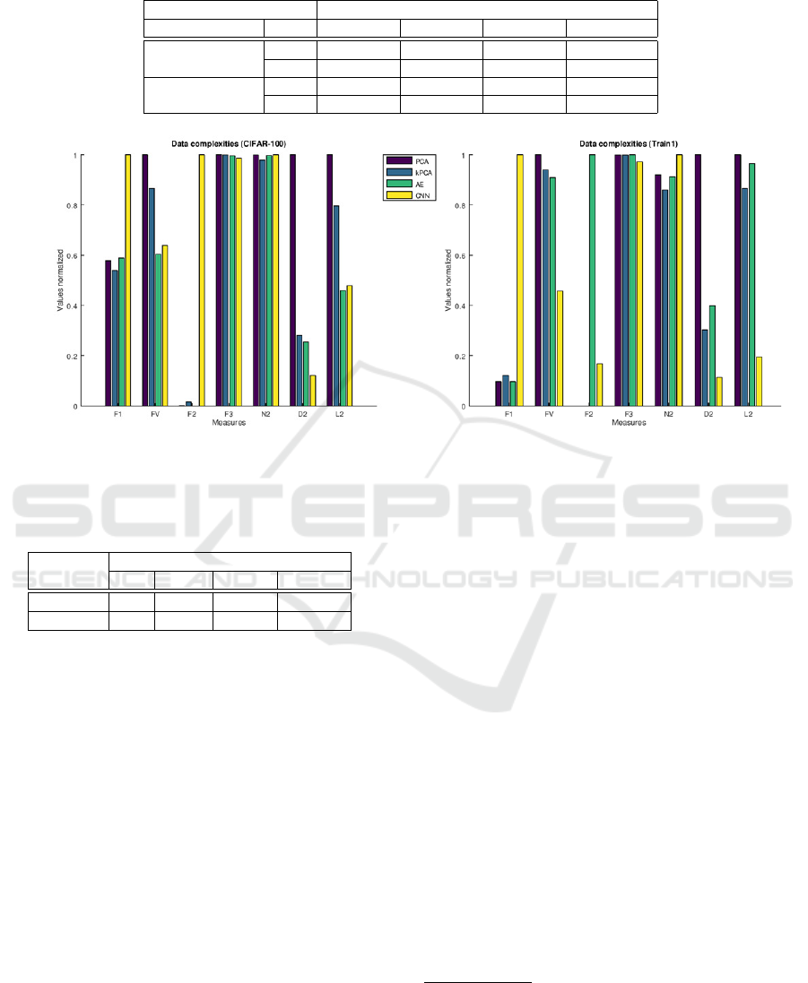
Table 2: The classification accuracy mean rates (%) (and standard deviation in parentheses) measured with the four extractors
for Train1 and Test1. Here the highest accuracy in each row is highlighted with a ? marker.
classification methods feature extraction methods
classifiers types PCA kPCA AE-features CNN-features
kNN k = 1 69.93 (0.56) 72.07 (0.36) 70.13 (0.61)
?
74.45 (0.50)
k = 3 68.72 (0.85) 71.53 (0.34) 69.08 (0.89)
?
75.80 (0.39)
SVM polyn. 52.91 (0.16) 65.13 (0.30) 65.92 (0.45)
?
80.58 (0.30)
(opts = ’-s 0 -t 1/2’) rbf 73.32 (0.40) 75.76 (0.41) 76.45 (0.37)
?
85.14 (0.25)
Figure 2: Plots comparing the four complexity measures obtained in the four subspaces developed from CIFAR-100 (left)
and Train1 (right). For ease of comparison, the complexity values measured in each of the four subspaces were divided into
the largest of the four values and then displayed graphically.
Table 3: The processing CPU-times (in seconds) measured
with the four extraction methods.
datasets feature extraction methods
PCA kPCA AE-feat. CNN-feat.
CIFAR-100 6.4 99.8 6,103.9 6.3
Train1 8.3 7,775.0 9,560.8 35.5
(in seconds) for each data set is the time obtained by
repeating the feature extraction several times and then
averaging it.
Table 3 presents a numerical comparison of the
processing CPU-times (in seconds). Here the times
recorded are the required CPU-times on a laptop com-
puter with a CPU Core(TM) i7-9750H speed of 2.60
GHz and RAM 16.0 GB, and operating on a Window
10 Home 64-bit platform.
In the results of the comparison, it can be observed
that the extractor of CNN-features requires a much
shorter processing CPU-time than the traditional non-
linear algorithms (i.e., kPCA) for the datasets used. In
particular, this result demonstrates that the extractor
can dramatically reduce processing time compared to
other network-based methods (e.g., AE-features).
However, it should be noted that extracting the
CNN-features requires a pretrained model. That is,
the CNN-features were obtained after training in the
CNN architecture using the pretrained model as an
initial weight matrix (i.e., after fine-tuning). In this
experiment, CIFAR-100 (train) was used for CIFAR
to obtain the pretrained model (# epochs is 100), and
Train2 was used for seismic data (# epochs is 300).
Then, the training time for these models was excluded
when counting the processing time in Table 3.
4.4 Experiment #2: Real-world Data
To further investigate the improvement, we extracted
patch data from real seismic wave image data and then
repeated the above classification. Our real seismic im-
ages were cited from Project Netherlands Offshore F3
Block - Complete
9
.
First, fault lines were marked manually after the
fault and normal patches were extracted from the real
seismic images
10
. For simple comparative analysis,
only ten seismic images were displayed with the fault
lines. Then, when extracting patches, the number of
patches on the larger side was adjusted to the smaller
side by randomly selecting them to prevent imbal-
ance between classes. A total of 52, 026(= 26, 013 +
26, 013) fault and non-fault patches were extracted
9
https://terranubis.com/datainfo/Netherlands-Offshore-
F3-Block-Complete
10
The work of assigning fault lines to real seismic wave
images should be done by human labelers using appropriate
tools, as was in ImageNet (Krizhevsky, A. et al., 2012).
Empirical Evaluation on Utilizing CNN-features for Seismic Patch Classification
171

Table 4: The classification accuracy mean rates (%) (and standard deviation in parentheses) measured with the four extractors
from the real seismic data. Here the highest accuracy in each row is highlighted with a ? marker.
classification methods feature extraction methods
classifiers types PCA kPCA AE-features CNN-features
kNN k = 1 92.47 (0.39) 93.10 (0.25) 86.33 (0.34)
?
95.49 (0.27)
k = 3 84.52 (0.46) 86.56 (0.42) 74.59 (0.43)
?
93.60 (0.15)
SVM polyn. 80.20 (0.47) 86.69 (0.45) 72.69 (0.00)
?
85.47 (0.42)
(’-s 0 -t 1/2 -c 10’) rbf 91.16 (0.27) 93.32 (0.29) 83.58 (0.00)
?
95.22 (0.24)
Table 5: The classification accuracy rates (%) obtained with
a fully-connected CNN and two HYBs.
classifiers synthetic data real data
CNN (fully-connected) 84.78 (0.28) 92.82 (0.16)
kNN (k = 1) 74.48 (0.32) 95.52 (0.19)
SVM (’-s 0 -t 2 -c 10’) 85.06 (0.23) 95.20 (0.21)
from the ten seismic images.
Next, the extracted patches were classified in the
four ways and the accuracy was compared. The eval-
uation here was conducted under the same conditions
as the experiments in Table 2, including all param-
eters for extracting CNN-features and learning the
classifiers. In particular, as recently was done in
(Cunha, A. et al., 2020), the pretrained model used
for CNN learning of synthetic data was used after
fine-tuning using the real-world patch data. Table 4
presents a numerical comparison of the classification
accuracy (mean and standard deviation in parenthe-
sis) rates (%). A random selection of 10, 000 (and
10, 000) patches was made for training (and test) data.
The assessment was repeated ten times and the results
obtained were averaged.
From Table 4, we can rediscover the results of ex-
periments very similar to those seen in Table 2. The
CNN-feature has again obtained the highest accuracy
in all classifications of the real-world patch data, as
in the previous synthetic data. This means that us-
ing CNN-features can meaningfully improve classi-
fication accuracy, and as discussed earlier, these im-
provements are attributed to the pretrained models. To
avoid repetition, among the experiments carried out in
Section 4.3, experiments other than classification ac-
curacy comparisons were omitted here.
Rather than using fully-connected CNNs, CNN-
features were categorizied using conventional (non-)
linear classifiers in the experiments. Thus, a compar-
ative analysis of these two recognition systems was
made. Table 5 presents a comparison of the classi-
fication accuracy (%) measured with three classifiers
for the synthetic and real-life seismic data. The as-
sessments performed under the conditions shown in
Table 4 were averaged ten times over.
In Table 5, it can be inspected that the accuracy of
HYB is superior to that of CNN: SVM is always good
and NN is good in real-life data. Through this ob-
servation we can conclude that by hybridizing CNN-
features with existing classifiers, we can improve the
classification of seismic patch data.
5 CONCLUSIONS
In an effort to design a pattern recognition system that
can be successfully utilized for seismic patch classi-
fication, a method of extracting feature vectors ob-
tained using CNNs was considered and empirically
evaluated. In this paper CNN-features were acquired
first using a pretrained CNN model and then used to
learn an existing classifier, such as SVM. This type
of classification is equivalent to replacing the FC lay-
ers of the CNN with the classifier. Simulation using
the experimental data confirmed that the features were
extracted at a relatively rapid rate and the classifica-
tion performance improved.
To answer the question why this hybrid is superior
to the original CNN, relationship between data com-
plexity and classification accuracy of input feature
vectors was investigated. We first identified the rela-
tionship using one public data that allows for visual
observation. This relationship was then rechecked
with experimental data. After extracting PCA-based
and CNN-based features, the data complexity and
classification accuracy were measured and compared
for these two types of features. From the comparison
obtained, it was observed that the discriminative abil-
ities of the latter outperformed that of the PCA-based.
Although it was demonstrated that the classifi-
cation can be improved by using the CNN-features,
the architecture was simply determined by referring
to the smallest structure that can express basic algo-
rithms. Thus, a comprehensive evaluation using var-
ious architectures such as GoogLeNet, ResNet, and
VGGNet for another structure of seismic wave data
remains a task to compare with the state-of-the-art
results in the domain. Also, empirical comparisons
were made with a limited number of feature extrac-
tors using seismic datasets that only represent an am-
ICPRAM 2021 - 10th International Conference on Pattern Recognition Applications and Methods
172

plitude attribute. In addition to these limitations, the
problem of theoretically investigating CNN-based ex-
tractors to extract powerful features remains unre-
solved.
ACKNOWLEDGEMENTS
This work was supported in part by the National
Key Research Development Program of China (No.
2018AAA0102201) and the National Natural Science
Foundation of China (No. 11671317).
REFERENCES
Alshazly, H., Linse, C., Barth, E., and Martinetz, T. (2019).
Handcrafted versus CNN features for ear recognition.
In Symmetry, volume 11, pages 1493.1–1493.27.
Athiwaratkun, B. and Kang, K. (2015). Feature repre-
sentation in convolutional neural networks. In arXiv
preprint arXiv:1507.02313.
Cano, J.-R. (2013). Analysis of data complexity measures
for classification. In Expert Systems with Applica-
tions, volume 40, pages 4820–4831.
Cunha, A., Pochet, A., Lopes, H., and Gattass, M. (2020).
Seismic fault detection in real data using transfer
learning from a convolutional neural network pre-
trained with synthetic seismic data. In Computers &
Geosciences, volume 135, pages 104344.1–104344.9.
Di, H., Wang, Z., and AlRegib, G. (2018). Seismic fault
detection from post-stack amplitude by convolutional
neural networks. In Proc of 80th EAGE Conference
and Exhibition, pages 1–5.
Donahue, J., Jia, Y., Vinyals, O., Hoffman, J., Zhang, N.,
Tzeng, E., and Darrell, T. (2014). Decaf: A deep con-
volutional activation feature for generic visual recog-
nition. In Proc of the 31st Int’l Conf. Mach. Learning
(ICML), pages 647–655.
Girshick, R., Donahue, J., Darrell, T., and Malik, J. (2014).
Rich feature hierarchies for accurate object detection
and semantic segmentation. In Proc of IEEE Conf on
CVPR (CVPR), pages 580–587.
Gogna, A. and Majumdar, A. (2019). Discriminative au-
toencoder for feature extraction: application to char-
acter recognition. In Neural Processing Letters, vol-
ume 49, pages 1723–1735.
Hertel, L., Barth, E., K ¨aster, T., and Martinetz, T. (2015).
Deep convolutional neural networks as generic feature
extractors. In Proc of Int’l Joint Conf on Neural Net-
works (IJCNN), pages 1–4.
Ho, T. K. and Basu, M. (2002). Complexity measures of su-
pervised classification problems. In IEEE Trans. Pat-
tern Anal. Mach. Intell., volume 24, pages 289–300.
Hung, L., Dong, X., and Clee, T. (2017). A scalable
deep learning platform for identifying geologic fea-
tures from seismic attributes. In The Leading Edge,
volume 36, pages 249–256.
Krizhevsky, A. (2009). Learning multiple layers of features
from tiny images. Univ. Toronto, Canada.
Krizhevsky, A., Sutskever, I., and Hinton, G. E. (2012). Im-
agenet classification with deep convolutional neural
networks. In Advances in Neural Information Pro-
cessing Systems (NIPS), pages 1097–1105.
Lin, T.-Y., RoyChowdhury, A., and Maji, S. (2015). Bilin-
ear CNN models for fine-grained visual recognition.
In Proc of Int’l Conf on CV (ICCV), pages 1449–1457.
Lorena, A. C., Garcia, L. P. F., Lehmann, J., Souto,
M. C. P., and Ho, T. K. (2018). How complex is
your classification problem? A survey on measuring
classification complexity. In ACM Comput. Surv., vol-
ume 52, pages 107:1–107:34.
Oquab, M., Bottou, L., Laptev, I., and Sivic, J. (2014).
Learning and transferring mid-level image represen-
tations using convolutional neural networks. In Proc
of IEEE Conf on CVPR (CVPR), pages 1717–1724.
Pochet, A., Diniz, P. H. B., Lopes, H., and Gattass, H.
(2019). Seismic fault detection using convolutional
neural networks trained on synthetic poststacked am-
plitude maps. In IEEE Geoscience and Remote Sens-
ing Letters, volume 16, pages 352–356.
Razavian, L., Azizpour, H., Sullivan, J., and Carlsson, S.
(2014). Cnn features off-the-shelf: an astounding
baseline for recognition. In Proc of IEEE Conf on
CVPR (CVPR), pages 512–519.
Sotoca, J. M., Mollineda, R. A., and S ´anchez, J. S. (2006).
A meta-learning framework for pattern classification
by means of data complexity measures. In Revista
Iberoamericana de Inteligencia Artificial, volume 10,
pages 31–38.
Sun, C., Shrivastava, A., Singh, S., and Gupta, A. (2017).
Revisiting unreasonable effectiveness of data in deep
learning era. In Proc of Int’l Conf on CV (ICCV),
pages 843–852.
Wang, Q. (2012). Kernel principal component analysis and
its applications in face recognition and active shape
models. In arXiv preprint arXiv:1207.3538.
Wang, Z., Di, H., Shafiq, M. A., Alaudah, Y., and AlRegib,
G. (2018). Successful leveraging of image processing
and machine learning in seismic structural interpre-
tation: A review. In The Leading Edge, volume 37,
pages 451–461.
Weimer, D., Scholz-Reiter, B., and Shpitalni, M. (2016).
Design of deep convolutional neural network archi-
tectures for automated feature extraction in industrial
inspection. In CIRP Annals - Manufacturing Technol-
ogy, volume 65, pages 417–420.
Zeiler, M. D. and Fergus, R. (2014). Visualizing and under-
standing convolutional networks. In Proc of European
Conf on CV (ECCV), pages 818–833.
Empirical Evaluation on Utilizing CNN-features for Seismic Patch Classification
173
