
Feature Extraction and Neural Network-based Analysis on
Time-correlated LiDAR Histograms
Gongbo Chen
1
, Pierre Gembaczka
1
, Christian Wiede
1
and Rainer Kokozinski
2
1
Fraunhofer Institute of Microelectronic Circuits and Systems (IMS), Finkenstrasse 61, Duisburg, Germany
2
University of Duisburg-Essen (UDE), Forsthausweg 2, Duisburg, Germany
Keywords: LiDAR, TCSPC, Histogram, Neural Network, Feature Extraction.
Abstract: Time correlated single photon counting (TCSPC) is used to obtain the time-of-flight (TOF) information
generated by single-photon avalanche diodes. With restricted measurements per histogram and the presence
of high background light, it is challenging to obtain the TOF information in the statistical histogram. In order
to improve the robustness under these conditions, the concept of machine learning is applied to the statistical
histogram. Using the multi-peak extraction method, introduced by us, followed by the neural-network-based
multi-peak analysis, the analysis and resources can be focused on a small amount of critical information in
the histogram. Multiple possible TOF positions are evaluated and the correlated soft-decisions are assigned.
The proposed method has higher robustness in allocating the coarse position (± 5 %) of TOF in harsh
conditions than the case using classical digital processing. Thus, it can be applied to improve the system
robustness, especially in the case of high background light.
1 INTRODUCTION
With the arising of advanced driver assistance
systems, sensor-based environment perception
becomes more and more important in automotive.
Therein, depth information is one of the key
parameters (Horaud et al., 2016). Light detection and
ranging (LiDAR) is one method to measuring
distance (Schwarz, 2010). Compare to other range
sensors, it provides the most depth range with high
distance resolution (Zaffar et al., 2018). Among the
detectors used in LiDAR systems, the single photon
avalanche diode (SPAD) is one solution with high
energy efficiency and excellent timing performance.
The SPAD-based LiDAR system determines the
distance by time-of-flight (TOF). However, the
SPAD can be easily triggered falsely by background
light because of its high sensitivity (Vornicu et al.,
2019). Therefore, one of the greatest interferences of
a SPAD-based LiDAR system is the background light
(Niclass et al., 2014).
Due to the interference, the TOF information
cannot be estimated from a single measurement. Time
correlated single photon counting (TCSPC) (Süss et
al., 2016) is a measuring method to obtain accurate
TOF information from a SPAD-based direct-TOF
system. The TCSPC accumulates plurality of
measurements and forms a statistical histogram in
order to distinguish the laser pulse from background
noise. The final TOF information is typically
obtained from the statistical histogram by classical
digital processing (CDP). The CDP estimates
distributions of noise and constructs noise-reduced
histograms. However, the performance of CDP
degrades significantly with the increasement of
background light and TOF (Kostamovaara et al.,
2015).
This paper focuses on TCSPC histograms
generated by the SPAD-based direct TOF flash
LiDAR system. The robustness of TOF prediction
can be improved by analysing unused information in
the TCSPC histograms. Considering the application
in automotive, where an approximation of the TOF
must be made and updated within restricted time and
under dynamic background light condition (Niclass et
al., 2014), the robustness of data processing methods
becomes therefore demanding. We propose a simple
method called multi-peak extraction (MPE) in
combination with a neural-network-based multi-peak
analysis (NNMPA) which assigns the soft-decision to
each extracted peak. The goal is to allocate the coarse
position (± 5 %) of the TOF in a noisy histogram.
Chen, G., Gembaczka, P., Wiede, C. and Kokozinski, R.
Feature Extraction and Neural Network-based Analysis on Time-correlated LiDAR Histograms.
DOI: 10.5220/0010185600170022
In Proceedings of the 9th International Conference on Photonics, Optics and Laser Technology (PHOTOPTICS 2021), pages 17-22
ISBN: 978-989-758-492-3
Copyright
c
2021 by SCITEPRESS – Science and Technology Publications, Lda. All rights reserved
17

The following content is structured as follows:
Section 2 covers the state-of-the-art works and
limitations in the field of LiDAR data processing.
Afterwards, the methodology including the
theoretical analysis and the structure of the neural
network is presented in section 3. Subsequently, the
used datasets for training, validation and testing are
described in section 4. Section 5 is devoted to the
result and discussion. In particular, the method
performance is discussed by means of the control
variable method and a comparison to the CDP is
carried out. Finally, section 6 summarizes the
outcome and outlines of the future work.
2 RELATED WORKS
Studies are carried out in different processing stages
of the LiDAR system to suppress the background
light. In this work, they are divided into three
categories:
2.1 On Hardware Stage
A bandpass filter can remove most of the background
light. However, remaining background light is still
significant. The coincidence detection (Perenzoni et
al., 2017) (Beer et al., 2018) is an effective approach
to prevent the SPADs from blocking out. This
approach involves several detectors in one pixel. The
detectors work in parallel. When two or more
detectors are triggered in a defined time interval, a
coincidence event is generated. The approach
performs well when the background light and the
laser echo are both high. In addition, time-gating
(Kostamovaara et al., 2015) improves the reception
rate of wanted signals by shortening the activation
duration of the SPADs. In order to activate the SPAD
at the right moment, the approach needs the
approximate position of the object as the prior-
knowledge, which is typically impractical in reality.
2.2 On Histograms
Using digital filters e.g. the matched-filter and the
center-of-mass algorithm are one of the classical
solutions applied on histograms. Besides, Tsai et al.
introduce a likelihood ratio test (LRT) based on a
probabilistic model (Tsai et al., 2018). They focus on
the precision of the measurements and report that the
standard deviation of the predicted distances is lower
than the center-of-mass algorithm under 100 MHz
background photon rate. However, the maximum
detection range is not sufficient in automotive, since
their experiment carried out only in 2 m.
2.3 On Point Cloud
The point cloud is the final output of the LiDAR
front-end. A good overview for applications of
machine learning methods on the point cloud can be
found in (Gargoum and El-Basyouny, 2017). One of
the pioneers analysing the point cloud data is
PointNet (Qi et al., 2017). They take the point sets
directly as input and provides a unified approach to
several 3D recognition tasks. These approaches can
improve the system robustness to a certain extent.
However, since they treat the LiDAR front-end as a
black box, errors introduced before the point cloud,
e.g. the background interference, cannot be handled
adequality.
3 METHODOLOGY
3.1 Multi-peak Extraction
A SPAD-based direct-TOF LiDAR front-end consists
of laser emitters, SPAD arrays, and corresponding
circuits and storage module. One measurement of the
first photon detection principle is described as
follows: A timer starts with the emission of the laser
pulse. Then, the laser pulse travels through the air and
is reflected by the object. Afterwards, the timer stops
with the detection of the first arrived photon. Finally,
the distance is calculated from the laser pulse
traveling time, i.e.:
2
(1)
where
is the arrival time of the first laser photon,
is the distance between the object and the
sensor, and is the speed of light. Since the triggering
event follows the Poisson process (Beer et al., 2016),
the probability density function (PDF) of the first
arriving photon is:
0
(2)
where
and
denote the photon rates of the
background and the laser pulse on the receiver side.
is equal to the sum of
and
.
is the laser
PHOTOPTICS 2021 - 9th International Conference on Photonics, Optics and Laser Technology
18
pulse width. In practice, the time axis is discrete due
to the sensor resolution
. Therefore, the
TCSPC histogram follows the probability mass
function (PMF)
, which can be obtained by
integrating (2) over
. An example of the ideal
PDF of the first received photon and the correlated
TCSPC histogram with specific settings is shown in
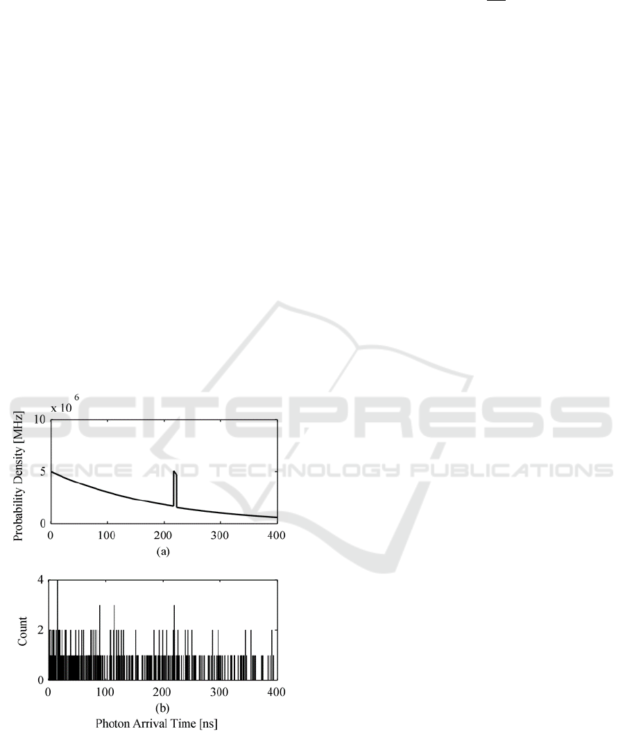
Figure 1. According to the optical statistics, it can be
interpreted that the TOF information corresponds to a
local maximum in a valid histogram, since the photon
intensity at the TOF moment is the superposition of
the laser and background photons. The rest of the
histogram contains only noise. However, as shown in
Figure 1, the measurement distribution will be sparse
and the jitter will be large in a time-restricted scenario
with certain amount of background noise. In this case,
selection of local maximums becomes critical.
Therefore, the MPE works as follows: 1) The
histogram is divided into adjacent regions, 2) in
each region, the local maximum
and its correlated
bin number b
n
will be extracted and coupled as a
region feature
,
, where ∈, 3) the
feature group
= {
,…,
} is formed as the
simplified representation of the complete histogram.
The number of extracted features is defined as:
Figure 1: (a) An example of the ideal probability density
function of the first received photon. (b) A correlated
TCSPC histogram. Where,
is equal to 312.5 ps,
is set to 216.67 ns, the background photon rate after
the bandpass filter is 5 MHz, the echo photon rate is 10
MHz,
is 5 ns, and the number of accumulated
measurements is 400 resulting in a frame rate of 25 Hz.
(3)
where in
is the measurement range and
is the
region width. All regions have the same
. After
obtaining
, the memory space for the complete
histogram can be released.
3.2 Multi-peak Analysis
In order to analyze the utility of
, the NNMPA is
designed. The NNMPA comprises a multi-
classification phase and a TOF recovery phase. In the
multi-classification phase, we construct a
fully-connected feed-forward neural network
(FNN). The FNN has one hidden layer. The learning
rate is set to 0.001. Additionally, L2 generalization
and drop-out layer are used to improve the
generalization. The FNN is trained and tested only by
the extracted local maximums {
,…,
}. The
actual TOF information in the histograms is
converted to categories as labels to supervise the
training process. Accordingly, the soft-decisions
{
,…,
} are calculated and assigned to local
maximums using the soft-max function. The local
maximum
having the highest score
will be
chosen as the final prediction. In the TOF recovery
phase, the TOF is calculated from the bin index
correlated to
.
4 DATASETS
In the scope of this work, two datasets are used:
4.1 Dataset 1
The first dataset is generated by a simulation tool
developed by Fraunhofer IMS. The dataset consists
of 600 histograms. The pulse width, the received laser
photon rate and the measurements in each histogram
is set to 5 ns, 10 MHz, and 400, respectively. The
simulated background photon rates (BPRs) after the
optical bandpass filter are 1, 2, 3, 4, 5 MHz and the
simulated TOF information are from 2.5 m to 57.5 m,
with an interval of 5 m. The simulated histograms are
evenly distributed under each combination of
aforementioned conditions. Dataset 1 is used for the
probability analysis of MPE and the evaluation of the
neural network.
Feature Extraction and Neural Network-based Analysis on Time-correlated LiDAR Histograms
19
4.2 Dataset 2
The second dataset originates from the LiDAR
system “OWL” developed by Fraunhofer IMS
(mentioned as OWL in the following context). It
consists of 120 histograms. The OWL is specified as
follows: the used lasers emit at 905 nm wavelength
with 75 W peak power, 10 kHz pulse repetition rate,
and 17.5 ns pulse width resulting in a mean optical
emission power of 11.25 mW. Each histogram
contains 400 single measurements. The histograms
are generated under BPR range of 3 – 10 MHz with
the object at 7.49 m, 17.35 m and 25.95 m. The BPR
is measured using OWL running in the counting
mode. Dataset 2 is used to validate the MPE and as
test dataset for the neural network.
5 RESULTS AND DISCUSSION
5.1 Performance of Multi-peak
Extraction
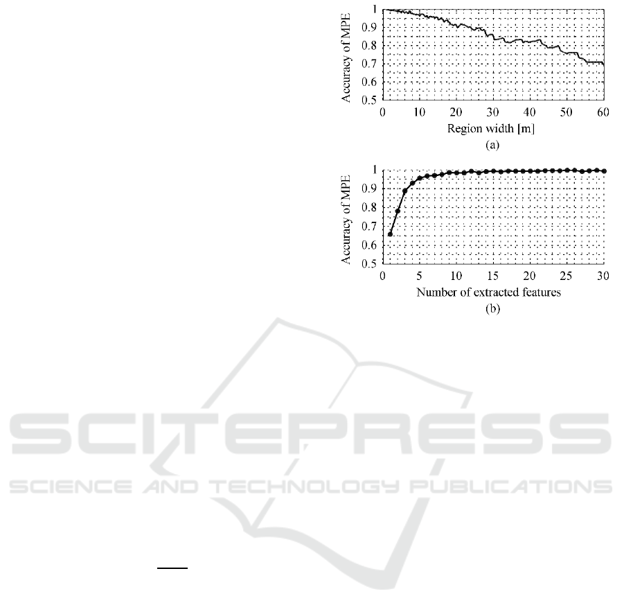
The most important factor of MPE is the region
width, which directly influences the extraction of
local maximums and the number of extracted local
maximums. The Monte-Carlo method is used on
dataset 1 to estimate the accuracy of the MPE
corresponding to each region width. The histograms
are filtered by a convolutional core C = {C(0), … ,
C(15)} before applying the MPE, where C(0) = …=
C(15) = 1. Figure 2 shows the evaluation result. The
accuracy of the MPE is defined as:
(4)
where
represents the number of
, which is
equal to the number of histograms.
represents
the number of true
. A true
must meet the
following condition: ∃
∈
, that:
15%
15%
(5)
As expected, the accuracy of MPE is inverse-
proportional to the region width. Due to
discontinuous
in the histograms of dataset 1, the
right part of the curve in Figure 2 (a) is jagged. As
shown in Figure 2 (b), the accuracy of MPE increases
rapidly in the initial period, and gradually stabilizes
with the increasing number of extracted features.
Figure 2: (a) Accuracy vs. region width on dataset 1. (b)
Accuracy vs. number of inputs on dataset 1. Since each
region width corresponds to one accuracy of MPE, while
each number of extracted features corresponds to one or
more region widths, the accuracy of MPE at each point in
(b) is obtained by averaging the accuracies corresponding
to the same number of extracted features.
In the scope of this work, instead of evaluating the
complete histogram (1200 bins), we extracted 12
region features (
= 4.91 m) for further processing,
resulting in a 121212 FNN. In this case,
is 97.83 % on dataset 1. Note that under the
harshest condition in dataset 1 (
equals to 57.5
m and BPR equals to 5 MHz), some histograms are
invalid, i.e. there is no peak at the target position. The
setting is further validated on dataset 2 and achieves
99.17 % of
.
5.2 Performance of Multi-peak
Analysis
The NNMPA is evaluated on the basis of dataset 1
and dataset 2. The performance is compared to the
CDP. The CDP in this work performs the same
preprocessing method (including the convolutional
core C and the noise subtraction algorithm) as the
NNMPA and uses the matched-filter to extract the
TOF. The FNN is trained on 70 % of dataset 1,
validated on the rest 30 % of dataset 1, and tested on
dataset 2. The error bound is set to ±5 % of the TOF.
By saving
and
as feature pairs and the
followed TOF recovery process, NNMPA preserves
PHOTOPTICS 2021 - 9th International Conference on Photonics, Optics and Laser Technology
20

the original resolution of the sensor, although the
resolution of the used neural network is low.
Table 1: Performance comparison of CDP and NNMPA
from
perspective on dataset 1.
D
TOF
[m]
Number of
histograms
CDP
(±5 %)
NNMPA
(±5 %)
2.5 50 88.00 % 92.00 %
7.5 50 82.00 % 94.00 %
12.5 50 100.00 % 98.00 %
17.5 50 90.00 % 92.00 %
22.5 50 88.00% 92.00 %
27.5 50 84.00 % 88.00 %
32.5 50 84.00 % 100.00 %
37.5 50 72.00 % 88.00 %
42.5 50 58.00 % 96.00 %
47.5 50 60.00 % 92.00 %
52.5 50 58.00 % 90.00 %
57.5 50 54. 00 % 88.00 %
Table 2: Performance comparison of CDP and NNMPA
from BPR perspective on dataset 1.
BPR
[MHz]
Number of
histograms
CDP
(±5 %)
NNMPA
(±5 %)
1 120 99.17 % 100.00 %
2 120 95.83 % 100.00 %
3 120 85.83 % 97.50 %
4 120 60.00 % 85.83 %
5 120 47.50 % 79.17 %
Table 3: Performance comparison between CDP and
NNMPA on dataset 2.
D
TOF
[m]
BPR
[MHz]
Number
of
histogram
s
CDP
(±5 %)
NNMPA
(±5 %)
7.49 3 – 8 40 87.50 % 100.00 %
17.35 5 – 10 40 70.00 % 77.50 %
25.95 3 – 8 40 62.50 % 85.00 %
The classification results on dataset 1 show that
the used feed-forward neural network achieves 94.52
% of training accuracy and 92.22 % of validation
accuracy. After further converting the classification
result to the
through the bin index, the NNMPA
obtains 92.5 % of overall accuracy on the dataset 1,
while the CDP obtains 77.67 % of accuracy. A
detailed comparison is given by Table 1 and Table 2.
In Table 1, dataset 1 is divided into 12 sub-groups
according to the
. Each group has 50 histograms
with the BPR range of 1 – 5 MHz. It can be observed
that, the NNMPA outperforms the CDP except in the
third sub-set, where the CDP has slightly higher
accuracy (2%) than the NNMPA. Moreover, as the
increases, the accuracy of CDP drops to 54.00
%, while the performance of NNMPA is relative
stable. This means that for distant objects (up to 57.5
m), the detection robustness of NNMPA is higher
than that of the CDP. In Table 2, dataset 1 is divided
into 5 sub-groups according to the BPR. Each group
has 120 histograms with the
range of 0 – 60 m.
The result shows that, under the presence of low BPR
(1 MHz), both methods perform well. However, the
accuracy of CDP decreases gradually with the
increase of the BPR. When the BPR reaches 5 MHz,
the accuracy of CDP is reduced to 47.50 %.
Compared with CDP, although the accuracy of
NNMPA decreases with increasing BPR as well, its
accuracy remains at 79.17%. In terms of dataset 1, the
NNMPA shows its superiority in detection range and
background light tolerance. The experiment on
dataset 2 leads to a similar conclusion as shown in
Table 3. An interesting fact is, that the NNMPA has
an adaptability to the unaware data even under higher
BPR (the training dataset has the BPR range of 1 – 5
MHz). However, its performance on the dataset with
the BPR range of 5 – 10 MHz has still evidently
deteriorated.
In summary, the features extracted by the MPE
are sufficient to reveal the TOF information in the raw
histogram in the experimented environments.
Furthermore, the NNMPA outperforms the CDP
especially for distant objects and under high
background light.
6 CONCLUSIONS
This paper focuses on exploring useful information
on TCSPC histograms in order to improve the
robustness of
prediction with restricted
measurements and high background light. We have
proposed a novel method called neural network based
multi-peak analysis (NNMPA) including the multi-
peak extraction (MPE), a compact feed-forward
neural network and the TOF recovery process. The
criteria of feature extraction in TCSPC histograms is
discussed and the new representation for 600
simulated histograms and 120 histograms generated
Feature Extraction and Neural Network-based Analysis on Time-correlated LiDAR Histograms
21

by the LiDAR system “OWL” is created. The
NNMPA on the new representation of the histogram
is applied and its utility is proved. In contrast to the
classical digital processing (CDP), the NNMPA
analyzes only a small amount of data from the
histogram and has a higher accuracy on allocating the
coarse position ( 5% ) of TOF information
especially in harsh conditions. Although the NNMPA
cannot improve the precision of the TOF prediction,
it can provide reliable proposals so that high-
precision methods only need to focus on the partial
histogram.
The future work can be summarized in the
following four aspects:
1) An implementation of the proposed approach on
LabView or on FPGAs and a runtime test for the
distance prediction can be carried out.
2) Instead of FNN, other machine learning
algorithms such as SVM, decision tree, and naïve
Bayesian theory can be applied for further
investigation of the characteristics of extracted
features.
3) The proposed approach must be verified and
analyzed on larger datasets.
4) A feedback mechanism can be implemented to
improve the measurement reliability.
REFERENCES
Beer, M., Haase, J. F., Ruskowski, J., & Kokozinski, R.
(2018). Background Light Rejection in SPAD-Based
LiDAR Sensors by Adaptive Photon Coincidence
Detection. Sensors, 18(12), 1–16.
https://doi.org/10.3390/s18124338
Beer, M., Hosticka, B. J., & Kokozinski, R. (2016, June).
SPAD-based 3D sensors for high ambient illumination.
In 2016 12th Conference on Ph.D. Research in
Microelectronics and Electronics (PRIME) (pp. 1–4).
IEEE. https://doi.org/10.1109/PRIME.2016.7519466
Gargoum, S., & El-Basyouny, K. (Eds.) (2017). Automated
Extraction of Road Features using LiDAR Data: A
Review of LiDAR applications in Transportation. In
International Conference on Transportation
Information and Safety (ICTIS)
Horaud, R., Hansard, M., Evangelidis, G., & Ménier, C.
(2016). An overview of depth cameras and range
scanners based on time-of-flight technologies. Machine
Vision and Applications, 27(7), 1005–1020.
https://doi.org/10.1007/s00138-016-0784-4
Kostamovaara, J., Huikari, J., Hallman, L., Nissinen, I.,
Nissinen, J., Rapakko, H., Avrutin, E., & Ryvkin, B.
(2015). On Laser Ranging Based on High-
Speed/Energy Laser Diode Pulses and Single-Photon
Detection Techniques. IEEE Photonics Journal, 7(2),
1–15. https://doi.org/10.1109/JPHOT.2015.2402129
Niclass, C., Soga, M., Matsubara, H., Ogawa, M., &
Kagami, M. (2014). A 0.18-$\mu$m CMOS SoC for a
100-m-Range 10-Frame/s 200$\,\times\,$96-Pixel
Time-of-Flight Depth Sensor. IEEE Journal of Solid-
State Circuits, 49(1), 315–330.
https://doi.org/10.1109/JSSC.2013.2284352
Perenzoni, M., Perenzoni, D., & Stoppa, D. (2017). A 64 x
64-Pixels Digital Silicon Photomultiplier Direct TOF
Sensor With 100-MPhotons/s/pixel Background
Rejection and Imaging/Altimeter Mode With 0.14%
Precision Up To 6 km for Spacecraft Navigation and
Landing. IEEE Journal of Solid-State Circuits, 52(1),
151–160. https://doi.org/10.1109/JSSC.2016.2623635
Qi, C. R., Su, H., Mo, K., & Guibas, L. J. (Eds.) (2017).
PointNet: Deep Learning on Point Sets for 3D
Classification and Segmentation. In IEEE Conference
on Computer Vision and Pattern Recognition (CVPR)
http://arxiv.org/pdf/1612.00593v2
Schwarz, B. (2010). Mapping the world in 3D. Nature
Photonics, 4(7), 429–430.
https://doi.org/10.1038/nphoton.2010.148
Süss, A., Rochus, V., Rosmeulen, M., & Rottenberg, X.
(Eds.) (2016). Benchmarking time-of-flight based
depth measurement techniques. SPIE OPTO.
Tsai, S.Y., Chang, Y.C., & Sang, T.H. (Eds.). (2018).
Spad LiDARs: Modeling and Algorithms. Icsict-2018:
Oct. 31-Nov. 3, 2018, Qingdao, China. IEEE Press.
http://ieeexplore.ieee.org/servlet/opac?punumber=854
0788
Vornicu, I., Darie, A., Carmona-Galan, R., & Rodriguez-
Vazquez, A. (2019). Compact Real-Time Inter-Frame
Histogram Builder for 15-Bits High-Speed ToF-
Imagers Based on Single-Photon Detection. IEEE
Sensors Journal, 19(6), 2181–2190.
https://doi.org/10.1109/JSEN.2018.2885960
Zaffar, M., Ehsan, S., Stolkin, R., & Maier, K. M. (Eds.)
(2018). Sensors, SLAM and Long-term Autonomy: A
Review. In NASA/ESA Conference on Adaptive
Hardware and Systems (AHS).
http://ieeexplore.ieee.org/servlet/opac?punumber=851
5683
PHOTOPTICS 2021 - 9th International Conference on Photonics, Optics and Laser Technology
22
