
Forecasting Air Pollution in Munich: A Comparison of MLR, ANFIS,
and SVM
Andreas Humpe
1a
, Lars Brehm
2b
and Holger Günzel
2c
1
University of Applied Sciences Munich, Schachenmeierstrasse 35, 80636 Munich, Germany
2
University of Applied Sciences Munich, Am Stadtpark 20, 81243 Munich, Germany
Keywords: Prediction Model, Air Pollution, Adaptive Neuro-fuzzy Inference System, Support Vector Machine, Multiple
Linear Regression.
Abstract: As motor vehicle air pollution is a serious health threat, there is a need for air quality forecasting to fulfil
policy requirements, and lower traffic induced air pollution. This article compares the performance of multiple
linear regressions, adaptive neuro-fuzzy inference systems, and support vector machines in predicting one-
hour ahead particulate matter, nitrogen oxides and ozone concentration in the City of Munich between 2014
and 2018. The models are evaluated with different performance measures in-sample and out-of-sample. The
results generally support earlier studies on forecasting air pollution and indicate that adaptive neuro-fuzzy
inference systems have the highest predictive power in terms of R-square for all pollutants. Furthermore,
ozone can be predicted best, whereas nitrogen oxides are the least predictive pollutants. One reason for the
different predictability might be rooted in the short lifetime of nitrogen oxides compared to ozone. The results
here should be of interest to regulators and municipal traffic managements alike who are interested in
predicting air pollution and improve urban air quality.
1 INTRODUCTION
It is generally recognized that motor vehicle air
pollution is a serious health threat. Motor vehicle
emissions include e.g. carbon monoxide (CO),
nitrogen oxides like NO or NO
2
, ozone (O
3
) or
particulate matter (PM10, PM2.5) (for a discussion
see inter alia Klæboe et al., 2000, Crüts et al., 2008,
Künzli et al., 2000 and Gössling et al., 2019).
Resulting health risks might be bronchitis,
asthma, lung cancer, cardiopulmonary diseases and
cardiopulmonary mortality (for a discussion see inter
alia Hoek et al., 2002, Pope et al. 2002 and Zhang et
al., 2013). Künzli et al., (2000) suggest that air
pollution is responsible for 6% of total deaths in
Europe and half of this can be attributed to motor
vehicle transport.
Although air quality has improved over the last
decades, there is scientific evidence that current
levels of air pollution are still too high (Lancet
Commission, 2017). As a result, there is a need for air
a
https://orcid.org/0000-0001-8663-3201
b
https://orcid.org/0000-0003-0810-3752
c
https://orcid.org/0000-0003-3410-1443
quality monitoring to fulfil legislative and policy
requirements in order to lower traffic-induced air
pollution by traffic control (Molina-Cabello et al.,
2019). In recent years, artificial intelligence (AI)
methods like artificial neural networks (ANN) or
decision trees (DT) have been applied to air quality
modelling and forecasting.
For instance, Pawlak et al., (2019) used ANNs to
forecast surface ozone concentration in central
Poland for the following day. They concluded that
ANNs can be used as a significant, effective tool to
predict extreme levels of ozone. Similarly, Molina-
Cabello et al., (2019) successfully applied
transferable neural networks to infer NO
2
and PM10
emissions in the city of Leicester, UK.
In addition, adaptive neuro-fuzzy inference
systems (ANFIS) models have been used to forecast
pollutants like nitrogen oxides (NOx), carbon dioxide
CO
2
or PM2.5 and PM10 by e.g. Ausati et al., (2016),
Mihalache et al., (2016) or Oprea et al., (2017).
Authors concluded that the ANFIS models perform
500
Humpe, A., Brehm, L. and Günzel, H.
Forecasting Air Pollution in Munich: A Comparison of MLR, ANFIS, and SVM.
DOI: 10.5220/0010184905000506
In Proceedings of the 13th International Conference on Agents and Artificial Intelligence (ICAART 2021) - Volume 2, pages 500-506
ISBN: 978-989-758-484-8
Copyright
c
2021 by SCITEPRESS – Science and Technology Publications, Lda. All rights reserved

well, also in comparison to other statistical or AI
models.
With the emergence of support vector machines
(SVM), researchers have applied SVMs to emission
forecasting as well. Lu et al., (2002) investigate air
pollutant parameter forecasting using support vector
machines and found them superior to ANNs in
predicting air quality parameters. In contrast, Luna et
al., (2014) compared ANNs and SVMs to predict
ozone concentration in Rio de Janeiro and found both
methods equally well suited for ozone forecasting.
Finally, Opera et al., (2017) used decision trees
(DT) to predict particulate matter and compared the
technique to ANNs. The results clearly showed that
ANNs are superior to DTs in predicting PM.
In summary, there are many studies investigating
the performance of different AI methods in
forecasting a variety of pollutants. However, most
studies have only used a short time-frame of e.g. one
year and focused on one or two pollutants
exclusively. Furthermore, in literature mixed
evidence exists on the performance of SVMs in
comparison to ANN or ANFIS methods. Most studies
have not evaluated the out-of-sample performance
and only relied on in-sample performance measures.
We therefore add to the literature by using an
extended time span of 5 years of hourly data and
comparing the one-hour forecast performance of
multiple linear regressions (MLR), adaptive neuro-
fuzzy inference systems (ANFIS) and support vector
machines (SVM) for five pollutants. The selection of
methods was thus based on literature. We also make
use of an extended time frame of four years in-sample
training (80%) and one year out-of-sample testing
(20%).
Therefore, the objective of this study is to develop
a one-hour forecasting model for different air
pollutants in the city of Munich between 2014 and
2018. Before the introduction of the pre-stage of the
low emission zone (LEZ) in 2008, many heavy-duty
trucks drove through the city centre of Munich (Qadir
et al., 2013). Following the pre-stage, the LEZ was
extended in the following months and only allowed
vehicles with emission requirement of Euro2, Euro3
and Euro4 to enter the inner city. In October 2010,
regulations were tightened further to only allow
vehicles with emission requirement Euro3, Euro4 and
higher to go through the LEZ area. The final stage was
4
https://www.muenchen.de/rathaus/home_en/
Environment-and-Health/Low_emission_zone.html
5
https://www.right-to-clean-air.eu/fileadmin/
Redaktion/Downloads/Laymans_report_ENG_Right_to_
clean_Air.pdf
introduced in October 2012 and merely allows
vehicles with Euro4 emission requirements to access
the LEZ area
4
. Research that analysed air quality
modelling and forecasting in Munich before or during
the introduction of the LEZ includes Hülsmann et al.,
(2014) and Fensterer (2014). They reported a
significant reduction in air pollution after the
introduction of the LEZ in the city of Munich.
We therefore analyse the predictability of air
pollution in Munich after the introduction of the final
stage of the LEZ. However, since 2019 there has been
an ongoing discussion regarding a diesel-driving ban
in Munich due to high particulate matter emissions
exceeding EU limits
5
. Our analysis will help to better
understand the current emotional discussion and
underpin it with facts.
2 MATERIAL AND METHODS
A short description of the material and methods that
were used in our analysis is given in the following
section.
2.1 Material
This study used hourly data of vehicle traffic, air
quality measurements, and meteorological data from
Munich, Germany. The dataset spans from
01.01.2014 to 31.12.2018 and therefore consists of
43,824 hours of traffic, air quality, and
meteorological data.
The traffic data was collected by the German
Federal Roads Agency (Bundesanstalt für
Straßenwesen)
6
for five major access roads to the city
of Munich. These motorways (A8 – München West,
A9 - Schwabing, A94 – München Riem, A96 –
München Laim, A995 – München Giesing) are
equipped with automatic traffic counting systems and
register all vehicles going to or leaving Munich.
The Bavarian State Office for the Environment
(Bayerisches Landesamt für Umwelt)
7
provided
hourly data for particulate matter (PM10 and PM2.5),
nitrogen monoxide (NO), ozone (O
3
) and nitrogen
dioxide (NO
2
) from five air measurement stations
located in Munich (Allach, Johanneskirchen,
6
https://www.bast.de/BASt_2017/DE/Verkehrstechnik/
Fachthemen/v2-verkehrszaehlung/Aktuell/zaehl_
aktuell_node.html
7
https://www.lfu.bayern.de/luft/immissionsmessungen/
messwertarchiv/index.htm
Forecasting Air Pollution in Munich: A Comparison of MLR, ANFIS, and SVM
501
Landshuter Allee, Lothstraße, Stachus). All five
pollutants are reported in μg/m
3
.
Precipitation, relative humidity, sunshine
duration, temperature, wind speed and wind direction
were available from the German Meteorological
Service (Deutscher Wetterdienst)
8
.
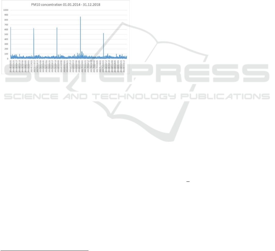
Furthermore, we include dummy variables for
New Year's Eve and working days because both show
variations in emissions. In particular, particulate
matter levels are ten times higher during New Year’s
Eve compared to average levels. The working day
dummy variables reflect different driving patterns
during public holidays and weekends. Figure 1 shows
the hourly PM10 concentration between 2014 and
2018 with extreme spikes of the pollutant during New
Year’s Eve.
Figure 1: Hourly PM10 concentration in μg/m3 between
01.01.2014 and 31.12.2018.
As traffic variable, we add all vehicles that are
going to or leaving Munich as recorded by the
automatic traffic counting system. For the five
pollutants, we calculate the average value of each
pollutant from the air measurement stations.
2.2 Methods
To evaluate the air forecasting performance of
artificial intelligence methods we compare adaptive
neuro-fuzzy inference systems (ANFIS) and support
vector machines (SVM) to multiple linear regressions
(MLR). The MLR as standard statistical method
serves as a benchmark for comparison. The selection
of ANFIS and SVM was based on recent literature in
atmospheric environmental sciences and artificial
intelligence (see inter alia Oprea et al., 2017; Ausati
et al., 2016; Quej et al., 2017; Pawlak et al., 2019 and
Mehrotra et al., 2020).
8
https://opendata.dwd.de/climate_environment/CDC/
observations_germany/climate/hourly/
2.2.1 Multiple Linear Regression
The multiple linear regression (MLR) was used as a
benchmark model for comparison with the support
vector machine (SVM) and the adaptive neuro-fuzzy
inference system (ANFIS). The MLR model can be
represented by:
⋯
(1)
where Y
i
is the i
th
observation of the dependent
variable Y, X
ji
is the i
th
observation of the j
th
independent variable, β
0
is the intercept, β
j
is the slope
coefficient of the j
th
independent variable and ε
i
represents the error term. The MLR assumes a linear
relationship between the dependent and the
independent variables.
2.2.2 Support Vector Machine
A support vector machine (SVM) is a supervised
learning algorithm from machine learning theory
(Vapnik, 1995). SVMs were originally developed for
classification problems, but can also be applied to
regression applications. We therefore use a SVM for
regression that is sometimes called a SVR model. The
SVM structure is not determined a priori but through
a model training process the input vectors are
selected. The training dataset is represented by:
(2)
Where x
i
is the input vector, d
i
is the desired value and
N is the total number of data patterns (He et al. 2014).
The regression function of the SVM is given by:
∗
(3)
where w
i
is a weight vector, b is a bias, and ϕ denotes
a nonlinear transfer function mapping the input
vectors into a high-dimension feature space. A
convex optimization problem with an e-insensitivity
loss function to obtain a solution to the following
equation was developed by Vapnik (1995):
:
1
2
‖
‖
∗
(4)
Subject to:
∗
∗
,1,2,…..,
∗
,1,2,…..,
,
∗
,1,2,…..,
(5)
Where ξ
i
and
∗
are slack variables that penalize
training errors by the loss function over the error
ICAART 2021 - 13th International Conference on Agents and Artificial Intelligence
502
tolerance ξ (He et al., 2014). Furthermore, C is a
positive trade-off parameter that determines the
degree of the empirical error in the equation (4). The
optimization problem in equation (4) is solved in a
dual form by using Lagrangian multipliers and
imposing the Karush-Kuhn-Tucker optimality
condition (see He et al. 2014). Input vectors that have
non-zero Lagrangian multipliers under the Karush-
Kuhn-Tucker condition are called support vectors as
they support the structure.
In our empirical analysis, we report the results of
linear SVMs. We have also estimated quadratic, cubic
and Gaussian SVMs and found very similar results to
the linear version, but estimation time was very long.
Hence, for practical reasons we make use of a linear
kernel function in our SVMs.
2.2.3 Adaptive Neuro-fuzzy Inference
System
An adaptive neuro-fuzzy inference system (ANFIS)
was first introduced by Jang (1993) and is a hybrid
model that combines a fuzzy with an artificial neural
network (ANN). It is a fuzzy inference system (FIS)
with distributed parameters (Quej et al., 2017). We
use a Sugeno first-order fuzzy model comparable to
Drake (2000). In a first-order Sugeno system, a
typical rule set with two fuzzy IF/THEN rules with
two inputs x and y and one output z is given by:
Rule 1:
(6)
If x is A
1
and y is B
1
, then
f
1
= p
1
x + q
1
y +
r
1
Rule 2:
(7)
If x is A
2
and y is B
2
, then
f
2
= p
2
x + q
2
y +
r
2
where p
1
, q
1
, r
1
and p
2
, q
2
, r
2
are the parameters in the
then-part of the first-order Sugeno fuzzy model (He
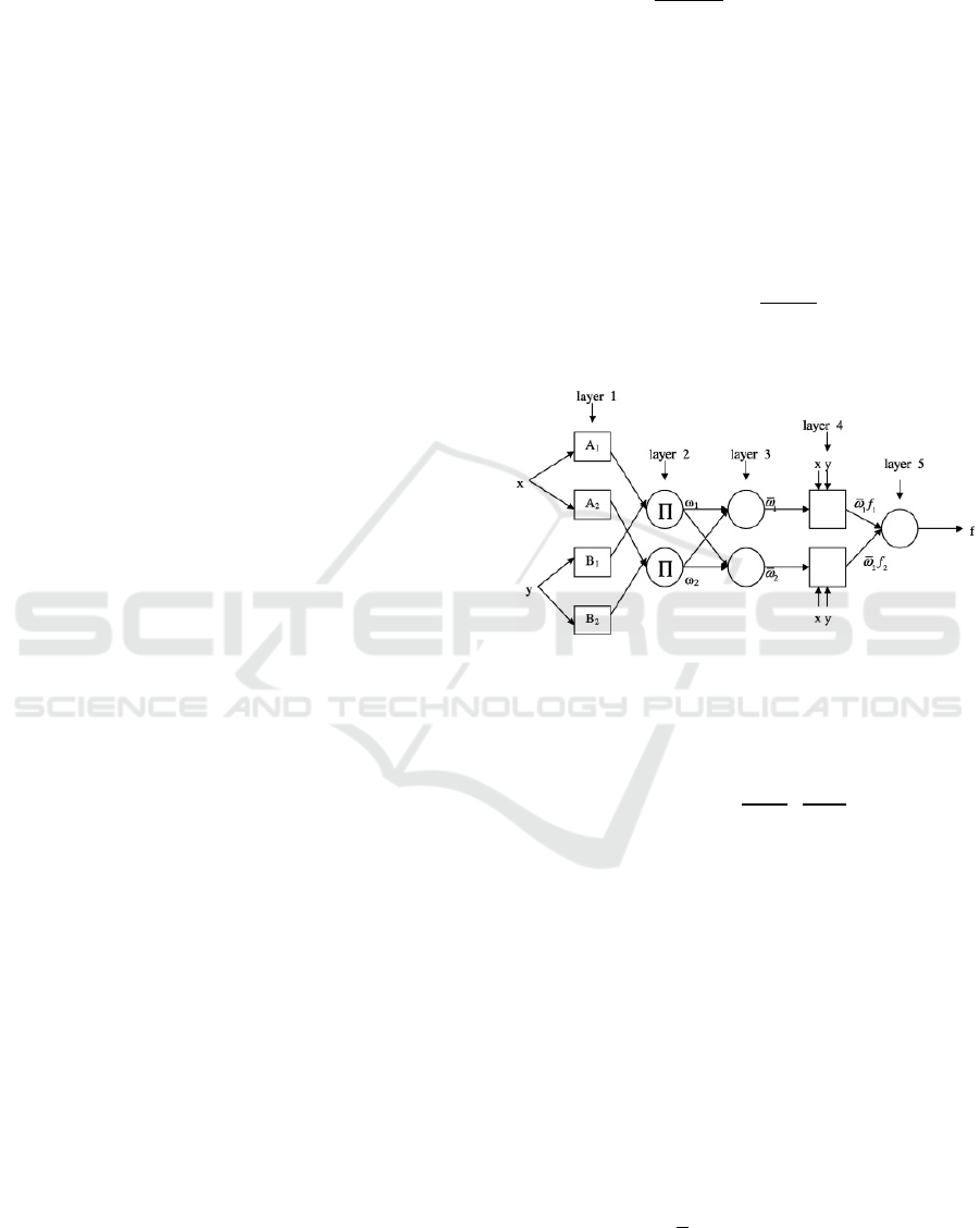
et al., 2014). The ANFIS consists of a five-layer
network (Wei et al., 2007) and the initial layer is
related to a fuzzy model (Ausati et al., 2016). Each
node i in the first layer represents a node function:
(8)
where x is the crisp input to the node i, and A
i
is the
fuzzy set associated with this node, characterized by
the shape of the membership functions (MFs). The
MFs can be e.g. triangular, trapezoidal, gaussian or
bell-shaped.
In the second layer (product layer) the rule
operator AND/OR is applied (Quej et al., 2017). The
outputs are obtained by multiplying ring layers with
the input layers:
∗
,1,2
(9)
In the third layer (normalized layer) the ratio of the i
th
rule’s strength compared to the sum of strength of all
rules is calculated:
,1,2
(10)
In the fourth layer (de-fuzzy layer), the weighted
output of each linear function is calculated:
(11)
where
is the output of the third layer and the final
parameters are p
i
, q
i
and r
i
.
In the fifth layer (total output layer) a single node
of total output with the sum of all inputs signals is
computed:
∑
∑
(12)
The figure below shows the ANFIS structure:
Figure 2: ANFIS structure (Guneri et al., 2011).
In our empirical analysis, we use two triangular
membership functions for each input variable in the
FIS. A triangular membership function is given by:
,
(13)
where a, b and c are the parameters that change the
shape of the triangular membership function with
maximum 1 and minimum 0 (Quej et al., 2017).
2.2.4 Model Evaluation
To evaluate the in- and out-of-sample forecasting
performance of the models, we use the means squared
error (MSE), the root mean squared error (RMSE), r-
squared (R2) and the mean absolute error (MAE).
The effect on MSE is more pronounced for large
errors in the forecasted values than for smaller errors
because the errors are squared. The MSE is calculated
as follows:
1
(14)
Where is the actual value and y is the predicted
output of the model.
Forecasting Air Pollution in Munich: A Comparison of MLR, ANFIS, and SVM
503
The square root of MSE gives RAMSE, which has
the same units as the forecasted values. The formula
for RMSE is given by:
∑
(15)
The MAE is a directionless method for comparing
forecasted values with realized outcomes in the data
(Hipni et al., 2013). MAE can be calculated by:
1
|
|
(16)
The R
2
is the ratio of the explained variation that can
be explained by the model and ranges between 0
(cannot explain any variation in the data) and 1 (can
explain the data variation completely). The R
2
is
given by:
1
∑
∑
(17)
To evaluate the model results, all four performance
measures are used and compared.
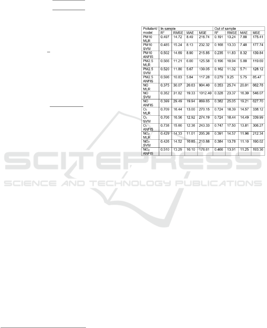
3 RESULTS
Table 1 reports the results of the in- and out-of-
sample performance measures of MLR, SVM and
ANFIS in forecasting PM10, PM2.5, NO, O
3
and
NO
2
. For in-sample results, the ANFIS model has the
highest R
2
and the lowest RAMSE/MSE for all
pollutants. Only for MAE do we find the lowest value
for PM10, PM2.5 and NO with the SVM, whereas for
O
3
and NO
2
the ANFIS models shows the lowest
MAE. Generally, the SVM
9
and MLR show similar
in-sample performance results. However, the ANFIS
tends to have the best performance in-sample for all
five pollutants. Ozone has the best in-sample
predictive power with a R
2
greater than 0.70 for all
three methods. The R
2
of NO is the lowest with values
below 0.40 for all models and is therefore the least
predictive pollutant in-sample.
For the out-of-sample results, we get a similar
picture as in-sample. The R
2
of the ANFIS is the
highest for PM10, PM2.5, NO, O
3
and NO
2
. ANFIS
also shows the lowest RAMSE/MSE for PM10,
PM2.5 and O
3
whereas the RAMSE/MSE for NO and
NO
2
has the lowest value for the SVM model. The
out-of-sample performance of MLR and SVM is
9
The number of support vectors are 11,968 for PM10;
10,085 for PM2.5; 17,649 for NO; 7,040 for O3 and
12,026 for NO2
again comparable, whereas the ANFIS model is
generally superior to MLR and SVM. Ozone can be
predicted best out-of-sample with a R
2
greater than
0.72 for all models. In contrast, PM10 and PM2.5 is
least predictive with a R
2
of approximately 0.20.
Table 1: Forecasting pollutants one hour ahead.
4 DISCUSSION
In contrast to MLR and ANFIS, a major advantage of
SVMs is that a relatively small sample might be
sufficient to build an effective calibrated model
(Balabin et al., 2011). However, in our case study of
Munich, the dataset is quite large and the small
sample advantage of SVMs cannot be exploited. This
might explain why the MLR and SVM perform very
similar in- and out-of-sample.
In recent years, particulate matter has been
reported as one of the most harmful air pollutants that
causes serious health problems especially to children
and elderly people (Oprea et al., 2017). Although the
R
2
indicates that only about 50% to 60% of the
variance in PM10 and PM2.5 can be explained by our
models, the ANFIS shows the highest R
2
. A
comparable R
2
between 50% and 60% has also been
reported by earlier studies with artificial neural
networks by e.g. Molina-Cabello (2019). Our results
are therefore in line with literature on the
predictability of particulate matter.
ICAART 2021 - 13th International Conference on Agents and Artificial Intelligence
504

Ozone is a secondary pollutant, as it is not directly
emitted by traffic, but produced through a chain of
photochemical reactions involving NOx, CO and
VOC (Volatile Organic Compounds). The
concentration of surface ozone is determined by a
combination of factors involved in its formation
(photochemical reactions), destruction (dry
deposition, chemical reactions) and transport (Pawlak
et al., 2019). Therefore, ozone is primarily formed on
warm summer days by solar radiation in combination
with the above mentioned pollutants. The relatively
long lifetime of ozone and its formation being
dependent on sunshine, causes a clear seasonal
pattern of ozone concentration over the year with a
spike in summer and a low during winter (Austin et
al., 2015). This might be the reason why ozone is
more predictable than the other pollutants.
In contrast to ozone, nitrogen oxides (NO, NO
2
)
are short-lived pollutants with a lifetime of 1 to 12
hours (Lorente et al., 2019). Nitrogen oxides react by
photochemical processing to form acid rain, ozone
and particulate matter. This could be the reason why
nitrogen oxides are the least predictable pollutants in
our sample.
As ozone and particulate matter concentration
depend on e.g. nitrogen oxides, some studies have
included these pollutants to better predict PM10,
PM2.5 and O
3
(see inter alia Ausati et al., 2016; Opera
et al., 2017 and Arsic et al., 2020). Future research
might therefore analyse the performance of our
models to forecast emissions in Munich by
incorporating NOx and CO as lagged predictors.
Future research in this area might include
additional artificial intelligence methods like long
short-term memory networks (LSTM). For instance,
Lin et al., (2019) used LSTM for PM10 forecasting
purposes.
5 CONCLUSIONS
This article compared the performance of multiple
linear regressions, adaptive neuro-fuzzy inference
systems and support vector machines in predicting
one-hour ahead particulate matter, nitrogen oxides
and ozone concentration in the City of Munich
between 2014 and 2018. The models were evaluated
with different performance measures in-sample and
out-of-sample. The results show that adaptive neuro-
fuzzy inference systems have the highest predictive
power in terms of R-square for all pollutants.
Furthermore, ozone can be predicted best, whereas
nitrogen oxides are the least predictive pollutants.
One reason for the different predictability might be
rooted in the short lifetime of nitrogen oxides
compared to ozone. As ozone and particulate matter
depend on nitrogen oxides, some research studies
have included these pollutants as lagged predictors.
Future research might therefore review our models
with lagged pollutants as predictor variables.
REFERENCES
Arsić, M., Mihajlović, I., Nikolić, D., Živković, Z., Panić,
P., 2020. Prediction of Ozone Concentration in
Ambient Air Using Multilinear Regression and the
Artificial Neural Networks Methods, Ozone: Science &
Engineering, 42:1, 79-88, DOI:
10.1080/01919512.2019.1598844.
Ausati, S., Amanollahi, J., 2016. Assessing the accuracy of
ANFIS, EEMD-GRNN, PCR, and MLR models in
predicting PM2.5, Atmospheric Environment, 142,
465-474.
Austin, E., Zanobetti, A., Coull, B., Schartz, J., Gold, D.,
Koutrakis, P., 2015. Ozone trends and their relationship
to characteristic weather patterns. Journal of Exposure
Science and Environmental Epidemiology, 25, 532–
542, DOI: 10.1038/jes.2014.45.
Balabin, R.M., Lomakina, E.I., 2011. Support vector
machine regression (LS-SVM) – an alternative to
artificial neural networks (ANNs) for the analysis of
quantum chemistry data?, Physical Chemistry
Chemical Physics, 13, 11710-11718, DOI:
10.1039/C1CP00051A.
Crüts, B., van Etten, L., Törnqvist, H., Blomberg, A.,
Sandström, T., Mills, N.L., Borm, P.J., 2008. Exposure
to diesel exhaust induces changes in EEG in human
volunteers. Particle and Fibre Toxicology, 5, 4.
Drake, J.T., 2000. Communications phase synchronization
using the adaptive network fuzzy inference system,
Ph.D. Thesis, New Mexico State University, Las
Cruces, New Mexico, USA.
Fensterer, V., Küchenhoff, H., Maier, V., Wichmann, H. ,
Breitner, S., Peters, A., Gu, J., Cyrys, J., 2014.
Evaluation of the Impact of Low Emission Zone and
Heavy Traffic Ban in Munich (Germany) on the
Reduction of PM10 in Ambient Air, International
Journal of Environmental Research and Public Health,
11(5), 5094–5112, Doi: 10.3390/ijerph110505094
Gössling, S., Humpe, A., Litman, T., Metzler, D., 2019.
Effects of Perceived Traffic Risks, Noise, and Exhaust
Smells on Bicyclist Behaviour: An Economic
Evaluation. Sustainability, 11, 408.
Guneri, A.F., Ertay, T., Yücel, A., 2011. An approach based
on ANFIS input selection and modeling for supplier
selection problem, Expert Systems with Applications,
38, 14907-14917.
He, Z., Wen, X., Liu, H. Du, J., 2014. A comparative study
of artificial neural network, adaptive neuro fuzzy
inference system and support vector machine for
forecasting river flow in the semiarid mountain region,
Journal of Hydrology, 509, 379-386.
Forecasting Air Pollution in Munich: A Comparison of MLR, ANFIS, and SVM
505

Hipni, A., El-shafie, A., Najah, A., Karim, O.A., Hussain,
A., Mukhlisin, M., 2013. Daily Forecasting of Dam
Water Levels: Comparing a Support Vector Machine
(SVM) Model With Adaptive Neuro Fuzzy Inference
System (ANFIS). Water Resource Management, 27,
3803-3823.
Hoek, G., Brunekreef, B., Goldbohm, S., Fischer, P., van
den Brandt, P.A., 2002. Association between mortality
and indicators of traffic-related air pollution in the
Netherlands: A cohort study. Lancet, 360, 1203–1209.
Hülsmann, F., Gerike, R., Ketzel, M., 2014. Modelling
traffic and air pollution in an integrated approach – the
case of Munich, Urban Climate, 10, 732-744.
Jang, J.S.R., 1993. ANFIS: adaptive-network-based fuzzy
inference system, IEEE Transactions on Systems, Man,
and Cybernetics, 23 (3), 665-685, doi:
10.1109/21.256541.
Klæboe, R., Kolbenstvedt, M., Clench-Aas, J., Bartonova,
A., 2000. Oslo traffic study—Part 1: An integrated
approach to assess the combined effects of noise and air
pollution on annoyance. Atmospheric Environment, 34,
4727–4736.
Künzli, N., Kaiser, R., Medina, S., Studnicka, M., Chanel,
O., Filliger, P., Herry, M., Horak, F., Jr.; Puybonnieux-
Texier, V.; Quénel, P., et al., 2000. Public-health impact
of outdoor and traffic-related air pollution: A European
assessment. Lancet, 356, 795–801.
Lin H., Jin J. and van den Herik J. (2019). Air Quality
Forecast through Integrated Data Assimilation and
Machine Learning.In Proceedings of the 11th
International Conference on Agents and Artificial
Intelligence - Volume 2: ICAART, ISBN 978-989-758-
350-6, pages 787-793. DOI:
10.5220/0007555207870793
Lorente, A., Boersma, K.F., Eskes, H.J., Veefkind, J.P., van
Geffen, J.H.G.M., de Zeeuw, M.B., Denier van der
Gon, H.A.C., Beirle, S., Krol, M.C., 2019.
Quantification of nitrogen oxides emissions from build-
up of pollution over Paris with TROPOMI. Scientific
Repeports, 9, 20033, DOI: 10.1038/s41598-019-56428-
5.
Lu, W., Wang, W., Leung, A.Y.T., Lo, S., Yuen, R.K.K.,
Xu, Z., Fan, H., 2002. Air pollutant parameter
forecasting using support vector machines, Proceedings
of the 2002 International Joint Conference on Neural
Networks. IJCNN'02 (Cat. No.02CH37290), Honolulu,
HI, USA, 2002, pp. 630-635 vol.1, doi:
10.1109/IJCNN.2002.1005545.
Luna, A.S., Paredes, M.L.L., de Oliveira, G.C.G., Correa,
S.M., 2014. Prediction of ozone concentration in
tropospheric levels using artificial neural networks and
support vector machine at Rio de Janeiro, Brazil,
Atmospheric Environment, 98, 98-104, DOI:
10.1016/j.atmosenv.2014.08.060.
Mehrotra A., Jaya Krishna R., Sharma D.P., 2020. Machine
Learning Based Prediction of PM 2.5 Pollution Level in
Delhi. In: Sharma H., Govindan K., Poonia R., Kumar
S., El-Medany W. (eds) Advances in Computing and
Intelligent Systems. Algorithms for Intelligent Systems.
Springer, Singapore. https://doi.org/10.1007/978-981-
15-0222-4_9
Mihalache, S.F., Popescu, M., 2016. Development of
ANFIS Models for PM Short-term Prediction. Case
Study. 8th International Conference on Electronics,
Computers and Artificial Intelligence (ECAI), Ploiesti,
2016, pp. 1-6, doi: 10.1109/ECAI.2016.7861073.
Molina-Cabello, M. A., Passow, B., Domínguez, E.,
Elizondo, D., Obszynska, J., 2019. Infering Air Quality
from Traffic Data Using Transferable Neural Network
Models, in: Advances in Computational Intelligence,
15th International Work-Conference on Artificial
Neural Networks, IWANN 2019, Gran Canaria, Spain,
June 12-14, 2019, Proceedings, Part I, pp.832-843,
DOI: 10.1007/978-3-030-20521-8_68.
Oprea, M., Popescu, M., Mihalache, S., Dragomir, E., 2017.
Data Mining and ANFIS Application to Particulate
Matter Air Pollutant Prediction. A Comparative Study,
in Proceedings of the 9th International Conference on
Agents and Artificial Intelligence - Volume 1:
ICAART, ISBN 978-989-758-220-2, pages 551-558.
DOI: 10.5220/0006196405510558
Pawlak, I., Jaroslawski, J., 2019. Forecasting of Surface
Ozone Concentration by Using Artificial Neural
Networks in Rural and Urban Areas in Central Poland,
Atmosphere, 10, 52.
Pope, C.A., III; Burnett, R.T.; Thun, M.J., Calle, E.E.,
Krewski, D., Ito, K., Thurston, G.D., 2002. Lung
cancer, cardiopulmonary mortality, and long-term
exposure to fine particulate air pollution. JAMA, 287,
1132–1141.
Qadir, R.M., Abbaszade, G., Schnelle-Kreis, J., Chow, J.C.,
Zimmermann, R., 2013. Concentrations and source
contributions of particulate organic matter before and
after implementation of a low emission zone in Munich,
Germany, Environmental Pollution, 175, 158-167.
Quej, V., Almorox, J. Arnaldo, J.A., Saito, L., 2017.
ANFIS, SVM and ANN soft-computing techniques to
estimate daily global solar radiation in a warm sub-
humid environment, Journal of Atmospheric and Solar-
Terrestrial Physics, 155, 62-70.
The Lancet Commission, 2017. The Lancet Commission on
Pollution and Health. Lancet, doi: 10.1016/S0140-
6736(17)32345-0.
Vapnik, V., 1995. The Nature of Statistical Learning
Theory, Springer, New York.
Wei, M., Bai, B., Sung, A.H., Liu, Q., Wang, J., Cather,
M.E., 2007. Predicting injection profiles using ANFIS,
Information Sciences, 177 (2), 4445-4461.
Zhang, K., Batterman, S., 2013. Air pollution and health
risks due to vehicle traffic. The Science of the total
environment, 450, 307–316.
ICAART 2021 - 13th International Conference on Agents and Artificial Intelligence
506
