
Self-supervised Dimensionality Reduction with Neural Networks and
Pseudo-labeling
Mateus Espadoto
1,3 a
, Nina S. T. Hirata
1 b
and Alexandru C. Telea
2 c
1
Institute of Mathematics and Statistics, University of S
˜
ao Paulo, Brazil
2
Department of Information and Computing Sciences, University of Utrecht, The Netherlands
3
Johann Bernoulli Institute, University of Groningen, The Netherlands
Keywords:
Dimensionality Reduction, Machine Learning, Neural Networks, Autoencoders.
Abstract:
Dimensionality reduction (DR) is used to explore high-dimensional data in many applications. Deep learning
techniques such as autoencoders have been used to provide fast, simple to use, and high-quality DR. How-
ever, such methods yield worse visual cluster separation than popular methods such as t-SNE and UMAP.
We propose a deep learning DR method called Self-Supervised Network Projection (SSNP) which does DR
based on pseudo-labels obtained from clustering. We show that SSNP produces better cluster separation than
autoencoders, has out-of-sample, inverse mapping, and clustering capabilities, and is very fast and easy to use.
1 INTRODUCTION
Analyzing high-dimensional data, a central task in
data science and machine learning, is challenging due
to the large size of the data both in the number of
observations and measurements recorded per obser-
vation (also known as dimensions, features, or vari-
ables). As such, visualization of high-dimensional
data has become an important, and active, field of
information visualization (Kehrer and Hauser, 2013;
Liu et al., 2015; Nonato and Aupetit, 2018; Espadoto
et al., 2019a).
Dimensionality reduction (DR) methods, also
called projections, have gained a particular place
in the set of visualization methods for high-
dimensional data. Compared to other techniques
such as glyphs (Yates et al., 2014), parallel coor-
dinate plots (Inselberg and Dimsdale, 1990), table
lenses (Rao and Card, 1994; Telea, 2006), and scat-
ter plot matrices (Becker et al., 1996), DR meth-
ods scale visually far better both on the number
of observations and dimensions, allowing the vi-
sual exploration of datasets having thousands of di-
mensions and hundreds of thousands of samples.
Many DR techniques have been proposed (Nonato
and Aupetit, 2018; Espadoto et al., 2019a), with
a
https://orcid.org/0000-0002-1922-4309
b
https://orcid.org/0000-0001-9722-5764
c
https://orcid.org/0000-0003-0750-0502
PCA (Jolliffe, 1986), t-SNE (Maaten and Hinton,
2008), and UMAP (McInnes and Healy, 2018) hav-
ing become particularly popular.
Neural networks, while very popular in machine
learning, are less commonly used for DR, with
self-organizing maps (Kohonen, 1997) and autoen-
coders (Hinton and Salakhutdinov, 2006) being no-
table examples. While having useful properties such
as ease of use, speed, and out-of-sample capability,
they lag behind t-SNE and UMAP in terms of good
visual cluster separation, which is essential for the in-
terpretation of the created visualizations. More recent
deep-learning DR methods include NNP (Espadoto
et al., 2020), which learns how to mimic existing DR
techniques, and ReNDA (Becker et al., 2020), which
uses two neural networks to accomplish DR.
DR methods aim to satisfy multiple functional
requirements (quality, cluster separation, out-of-
sample support, stability, inverse mapping) and non-
functional ones (speed, ease of use, genericity). How-
ever, to our knowledge, none of the existing meth-
ods scores well on all such criteria (Espadoto et al.,
2019a). In this paper, we propose to address this
by a new DR method based on a single neural net-
work trained with a dual objective, one of reconstruct-
ing the input data, as in a typical autoencoder, and
the other of data classification using pseudo-labels
cheaply computed by a clustering algorithm to in-
troduce neighborhood information, since intuitively,
Espadoto, M., Hirata, N. and Telea, A.
Self-supervised Dimensionality Reduction with Neural Networks and Pseudo-labeling.
DOI: 10.5220/0010184800270037
In Proceedings of the 16th International Joint Conference on Computer Vision, Imaging and Computer Graphics Theory and Applications (VISIGRAPP 2021) - Volume 3: IVAPP, pages 27-37
ISBN: 978-989-758-488-6
Copyright
c
2021 by SCITEPRESS – Science and Technology Publications, Lda. All rights reserved
27

clustering gathers and aggregates fine-grained dis-
tance information at a higher level, telling how groups
of samples are similar to each other (at cluster level),
and this aggregated information helps us next in pro-
ducing projections which reflect this higher-level sim-
ilarity.
Our method aims to jointly cover all the following
characteristics, which, to our knowledge, is not yet
achieved by existing DR methods:
Quality (C1). We provide better cluster separation
than standard autoencoders, and close to state-of-the-
art DR methods, as measured by well-known metrics
in DR literature;
Scalability (C2). Our method can do inference in lin-
ear time in the number of dimensions and observa-
tions, allowing us to project datasets of up to a mil-
lion observations and hundreds of dimensions in a few
seconds using commodity GPU hardware;
Ease of Use (C3). Our method produces good results
with minimal or no parameter tuning;
Genericity (C4). We can handle any kind of high-
dimensional data that can be represented as real-
valued vectors;
Stability and Out-of-Sample Support (C5). We
can project new observations for a learned projection
without recomputing it, in contrast to standard t-SNE
and any other non-parametric methods;
Inverse Mapping (C6). We provide, out-of-the-
box, an inverse mapping from the low- to the high-
dimensional space;
Clustering (C7). We provide, out-of-the-box, the
ability to learn how to mimic clustering algorithms,
by assigning labels to unseen data.
We structure our paper as follows: Section 2
presents the notation used and discusses related work
on dimensionality reduction, Section 3 details our
method, Section 4 presents the results that support our
contributions outlined above, Section 5 discusses our
proposal, and Section 6 concludes the paper.
2 BACKGROUND
We start with a few notations. Let x = (x
1
, . . . , x
n
),
x
i
∈ R, 1 ≤ i ≤ n be a n-dimensional (nD) real-valued
sample, and let D = {x
i
}, 1 ≤ i ≤ N be a dataset of N
samples. D can be seen as a table with N rows (sam-
ples) and n columns (dimensions). A DR, or projec-
tion, technique is a function
P : R
n
→ R
q
, (1)
where q n, and typically q = 2. The projection
P(x) of a sample x ∈ D is a qD point p ∈ R
q
.
Projecting a set D yields thus a qD scatter plot, which
we denote next as P(D). The inverse of P, denoted
P
−1
(p), maps a qD point to the high-dimensional
space R
n
.
Dimensionality Reduction. Tens of DR methods
have been proposed in the last decades, as extensively
described and reviewed in various surveys (Hoffman
and Grinstein, 2002; Maaten and Postma, 2009; En-
gel et al., 2012; Sorzano et al., 2014; Liu et al., 2015;
Cunningham and Ghahramani, 2015; Xie et al., 2017;
Nonato and Aupetit, 2018; Espadoto et al., 2019a).
Below we only highlight a few representative ones,
referring for the others to the aforementioned surveys.
Principal Component Analysis (Jolliffe, 1986)
(PCA) has been widely used for many decades due
to its simplicity, speed, and ease of use and interpreta-
tion. PCA is also used as pre-processing step for other
DR techniques that require the data dimensionality to
be not too high (Nonato and Aupetit, 2018). PCA is
highly scalable, easy to use, predictable, and has out-
of-sample capability. Yet, due to its linear and global
nature, PCA lacks on quality, especially for data of
high intrinsic dimensionality, and is thus worse for
data visualization tasks related to cluster analysis.
The methods of the Manifold Learning family,
such as MDS (Torgerson, 1958), Isomap (Tenenbaum
et al., 2000) and LLE (Roweis and Saul, 2000) with
its variations (Donoho and Grimes, 2003; Zhang and
Zha, 2004; Zhang and Wang, 2007) try to map to
2D the high-dimensional manifold on which data is
embedded, and can capture nonlinear data structure.
These methods are commonly used in visualization
and they generally yield higher quality results than
PCA. However, these methods can be hard to tune, do
not have out-of-sample capability, do not work well
for data that is not restricted to a 2D manifold, and
generally scale poorly with dataset size.
Force-directed methods such as LAMP (Joia et al.,
2011) and LSP (Paulovich et al., 2008) are popular in
visualization and have also been used for graph draw-
ing. They can yield reasonably high visual quality,
good scalability, and are simple to use. However, they
generally lack out-of-sample capability. In the case of
LAMP, there exists a related inverse projection tech-
nique, iLAMP (Amorim et al., 2012), however, the
two techniques are actually independent and not part
of a single algorithm. Clustering-based methods, such
as PBC (Paulovich and Minghim, 2006), share many
of the characteristics of force-directed methods, such
as reasonably good quality and lack of out-of-sample
capability.
The SNE (Stochastic Neighborhood Embedding)
family of methods, of which t-SNE (Maaten and Hin-
ton, 2008) is arguably the most popular, have the key
IVAPP 2021 - 12th International Conference on Information Visualization Theory and Applications
28
Table 1: Summary of DR techniques and their characteristics.
Characteristic
Technique Quality Scalability Ease of use Genericity Out-of-sample Inverse mapping Clustering
PCA low high high high yes yes no
MDS mid low low low no no no
Isomap mid low low low no no no
LLE mid low low low no no no
LAMP mid mid mid high no no no
LSP mid mid mid high no no no
t-SNE high low low high no no no
UMAP high high low high yes no no
Autoencoder low high high low yes yes no
ReNDA mid low low mid yes no no
NNP high high high high yes no no
SSNP high high high high yes yes yes
ability to visually segregate similar samples, thus be-
ing very good for cluster analysis. While praised
for high visual quality, t-SNE has a (high) complex-
ity of O(N
2
) in sample count, is very sensitive to
small data changes, can be hard to tune (Wattenberg,
2016), and has no out-of-sample capability. Sev-
eral refinements of t-SNE improve speed, such as
tree-accelerated t-SNE (Maaten, 2014), hierarchical
SNE (Pezzotti et al., 2016), and approximated t-
SNE (Pezzotti et al., 2017), and various GPU accel-
erations of t-SNE (Pezzotti et al., 2020; Chan et al.,
2018). Yet, these methods require quite complex
algorithms, and still largely suffer from the afore-
mentioned sensitivity, tuning, and out-of-sample is-
sues. Uniform Manifold Approximation and Pro-
jection (UMAP) (McInnes and Healy, 2018) gener-
ates projections with comparable quality to t-SNE but
much faster, and with out-of-sample capability. How-
ever, UMAP shares some disadvantages with t-SNE,
namely the sensitivity to small data changes and pa-
rameter tuning difficulty.
Deep Learning. Autoencoders (AE) (Hinton and
Salakhutdinov, 2006; Kingma and Welling, 2013) aim
to generate a compressed, low-dimensional represen-
tation on their bottleneck layers by training the net-
work to reproduce its high-dimensional inputs on its
outputs. Autoencoders produce results comparable to
PCA on the quality criterion. However, they are easy
to set up, train, and use, are easily parallelizable, and
have out-of-sample and inverse mapping capabilities.
The ReNDA method (Becker et al., 2020) is a
deep learning approach that uses two networks, im-
proving on earlier work from the same authors. One
network implements a nonlinear generalization of
Fisher’s Linear Discriminant Analysis (Fisher, 1936);
the other network is an autoencoder used as a regular-
izer. ReNDA scores well on predictability and has
out-of-sample capability. However, it requires pre-
training of each individual network and scalability is
quite low.
Recently, Espadoto et al. (Espadoto et al., 2020)
proposed Neural Network Projections (NNP), where
a training subset D
s
⊂ D is selected and projected by
any DR method to yield a so-called training projec-
tion P(D
s
) ⊂ R
2
. D
s
is fed into a regression neural
network which is trained to output a 2D scatter plot
P
nn
(D
s
) ⊂ R
2
by minimizing the error between P(D
s
)
and P
nn
(D
s
). The trained network then projects un-
seen data by means of 2-dimensional, non-linear re-
gression. NNP is very fast, simple to use, generic,
and stable. However, the results show fuzzier clus-
ter separation (lower quality) than the training projec-
tions, and cannot do inverse projections. The NNInv
technique (Espadoto et al., 2019b), proposed by the
same authors, provides inverse projection capability,
but this requires setting up, training, and using a sep-
arate network.
Table 1 shows a summary of the aforementioned
DR techniques and how they fare with respect to each
characteristic. The last row highlights SSNP, our
technique, which we describe next.
Step 1: Label assignment
In: Clustering algo, D
tr
Out: Y
tr
Clustering (K-means, Affinity Propagation, DBSCAN, etc)
Ground Truth labels
Step 2: Training
In: D
tr
, Y
tr
Out: Trained network
Stochastic Gradient Descent
Joint optimization of classifier and reconstruction targets
Step 3: Assembly of final networks
In: Trained network
Out: N
P
, N
I
, N
C
Dismantle trained network
Construct final networks based on trained layers
Step 4: Inference
In: D→N
P
P(D)→N
I
D→N
C
Out: N
P
→P(D) N
I
→D N
C
→ Y
Networks trained and ready to use for
Direct projection, inverse projection and clustering
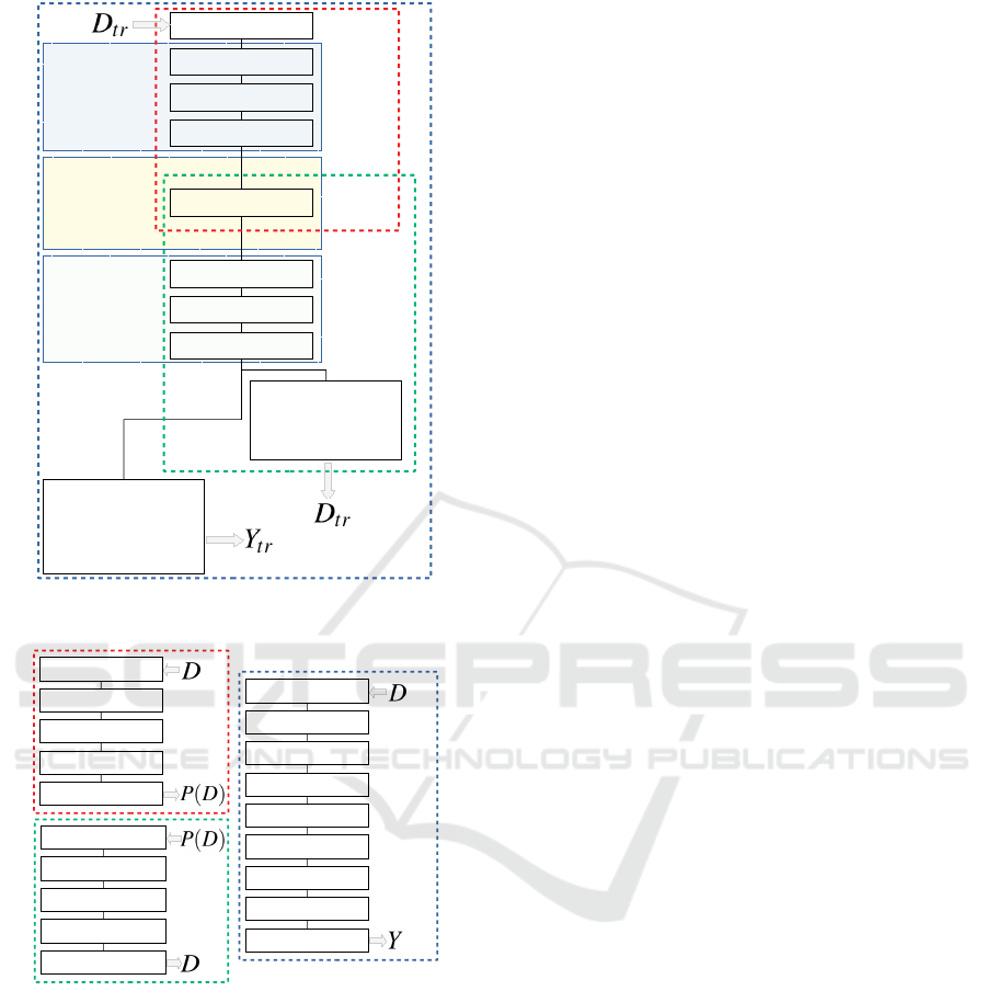
Figure 1: SSNP training-and-inference pipeline.
Self-supervised Dimensionality Reduction with Neural Networks and Pseudo-labeling
29
Encoder layers
Activation: ReLU
Init: Glorot Uniform
Bias: constant 0.0001
Embedding layer
Activation: Linear
Init: Glorot Uniform
Bias: constant 0.0001
L2: 0.5
Decoder layers
Activation: ReLU
Init: Glorot Uniform
Bias: constant 0.0001
Dense layer: 512 units
Input: n-dimensional
Dense layer: 128 units
Dense layer: 32 units
Dense layer: 2 units
Dense layer: 512 units
Dense layer: 128 units
Dense layer: 32 units
Classifier output:
k classes
Softmax activation
Categorical cross entropy loss
Reconstruction output:
n-dimensional
Sigmoid activation
Binary cross entropy loss
Direct
Projection
N
P
Inverse
Projection
N
I
Clustering
N
C
Figure 2: SSNP network architecture used for training.
Dense layer: 512 units
Input: n-dimensional
Dense layer: 128 units
Dense layer: 32 units
Output: 2-dimensional
Projection
Network
N
P
Input: 2-dimensional
Dense layer: 512 units
Dense layer: 128 units
Dense layer: 32 units
Inverse
Mapping
Network
N
I
Output: n-dimensional
Dense layer: 512 units
Input: n-dimensional
Dense layer: 128 units
Dense layer: 32 units
Dense layer: 2 units
Dense layer: 512 units
Dense layer: 128 units
Dense layer: 32 units
Clustering
Network
N
C
Output: k classes
Figure 3: Three SSNP networks used during inference.
3 METHOD
As stated in Section 2, autoencoders have desirable
DR properties (simplicity, speed, out-of-sample and
inverse mapping capabilities), but create projections
of lower quality than, e.g., t-SNE and UMAP. We
believe that the key difference is that autoencoders
do not use neighborhood information during training,
while t-SNE and UMAP (obviously) do that. This
raises the following questions: Could autoencoders
produce better projections if using neighborhood in-
formation? and, if so, How to inject neighborhood
information during autoencoder training? Our tech-
nique answers both questions by using a network ar-
chitecture with a dual optimization target. First, we
have a reconstruction target, exactly as in standard au-
toencoders; next, we use a classification target based
on pseudo-labels assigned by some clustering algo-
rithm e.g. K-means (Lloyd, 1982), Agglomerative
Clustering (Kaufman and Rousseeuw, 2005), or any
other way of assigning labels, including using “true”
ground-truth labels if available.
Our key idea is that labels –ground-truth or given
by clustering – are a high-level similarity measure
between data samples which can be used to infer
neighborhood information, i.e., same-label data are
more similar than different-label data. Since classi-
fiers seek to learn a representation that separates input
data based on labels, by adding an extra classifier tar-
get to an autoencoder, we learn how to project data
with better cluster separation than standard autoen-
coders. We call our technique Self-Supervised Neural
Projection (SSNP).
SSNP first takes a training set D
tr
⊂ D and assigns
to it pseudo-labels Y
tr
∈ Z by using some clustering
technique. We then take samples (x ∈ D
tr
, y ∈ Y
tr
) to
train a neural network with two target functions, one
for reconstruction, other for classification, which are
then added together to form a joint loss. The errors
from this joint loss are then back-propagated to the
entire network, during training. This network (Fig-
ure 2) contains a two-unit bottleneck layer, same as
an autoencoder, used to generate the 2D projection
when in inference mode. After training, we ‘split’
the trained layers of the network to create three new
networks for inference: a projector N
p
(x), an in-
verse projector N
i
(p) and, as a by-product, a classi-
fier N
c
(x), which mimics clustering algorithm used
to create Y
tr
(see Figure 3). The entire training-and-
inference operation of SSNP is summarized in Fig-
ure 1.
4 RESULTS
To evaluate SSNP’s performance we propose several
experiments to compare it with other DR techniques
using different datasets. We select the following
evaluation metrics, which are widely used in the
projection literature:
Trustworthiness (T ) (Venna and Kaski, 2006).
Measures the fraction of close points in D that are
also close in P(D). T tells how much one can trust
that local patterns in a projection, e.g. clusters,
represent actual patterns in the data. In the definition
IVAPP 2021 - 12th International Conference on Information Visualization Theory and Applications
30

Table 2: Projection quality metrics. Right column gives the metric ranges, with optimal values marked in bold.
Metric Definition Range
Trustworthiness (T ) 1 −
2
NK(2n−3K−1)
∑
N
i=1
∑
j∈U
(K)
i
(r(i, j) − K) [0, 1]
Continuity (C) 1 −
2
NK(2n−3K−1)
∑
N
i=1
∑
j∈V
(K)
i
(ˆr(i, j) − K) [0, 1]
Neighborhood hit (NH)
1
N
∑
y∈P(D)
y
l
k
y
k
[0, 1]
Shepard diagram correlation (R) Spearman’s ρ of (kx
i
− x
j
k, kP(x
i
) − P(x
j
)k), 1 ≤ i ≤ N, i 6= j [0, 1]
(Table 2), U
(K)
i
is the set of points that are among the
K nearest neighbors of point i in the 2D space but not
among the K nearest neighbors of point i in R
n
; and
r(i, j) is the rank of the 2D point j in the ordered-set
of nearest neighbors of i in 2D. We choose K = 7, in
line with (Maaten and Postma, 2009; Martins et al.,
2015);
Continuity (C) (Venna and Kaski, 2006). Measures
the fraction of close points in P(D) that are also close
in D. In the definition (Table 2), V
(K)
i
is the set of
points that are among the K nearest neighbors of
point i in R
n
but not among the K nearest neighbors
in 2D; and ˆr(i, j) is the rank of the R
n
point j in the
ordered set of nearest neighbors of i in R
n
. As with
T , we choose K = 7;
Neighborhood Hit (NH) (Paulovich et al., 2008).
Measures how well-separable labeled data is in a
projection P(D), in a rotation-invariant fashion,
from perfect separation (NH = 1) to no separation
(NH = 0). NH is the number y
l
k
of the k nearest
neighbors of a point y ∈ P(D), denoted by y
k
, that
have the same label as y, averaged over P(D). In this
paper, we used k = 3;
Shepard Diagram Correlation (R) (Joia et al.,
2011). The Shepard diagram is a scatter plot of the
pairwise distances between all points in P(D) vs the
corresponding distances in D. The closer the plot
is to the main diagonal, the better overall distance
preservation is. Plot areas below, respectively above,
the diagonal show distance ranges for which false
neighbors, respectively missing neighbors, occur. We
measure how close a Shepard diagram is to the ideal
main diagonal line by computing its Spearman rank
correlation R. A value of R = 1 indicates a perfect
(positive) correlation of distances;
We next show how SSNP performs on differ-
ent datasets when compared to t-SNE, UMAP, au-
toencoders, and NNP. We use different algorithms to
generate pseudo-labels, and also use ground-truth la-
bels. For conciseness, we name SSNP variants using
K-means, agglomerative clustering and ground-truth
labels as SSNP(Km), SSNP(Agg) and SSNP(GT),
respectively. We use two types of datasets: syn-
thetic blobs and real-world data. The synthetic blobs
datasets are sampled from a Gaussian distribution
where we vary the number of dimensions (100 and
700), the number of cluster centers (5 and 10), and use
increasing values of the standard deviation σ. This
yields datasets with cluster separation varying from
very sharp to fuzzy clusters. All synthetic datasets
have 5K samples.
Real-world datasets are selected from publicly
available sources, matching the criteria of being
high-dimensional, reasonably large (thousands of
samples), and having a non-trivial data structure:
MNIST (LeCun and Cortes, 2010). 70K samples of
handwritten digits from 0 to 9, rendered as 28x28-
pixel gray scale images, flattened to 784-element
vectors;
Fashion MNIST (Xiao et al., 2017). 70K samples
of 10 types of pieces of clothing, rendered as 28x28-
pixel gray scale images, flattened to 784-element
vectors;
Human Activity Recognition (HAR) (Anguita et al.,
2012). 10299 samples from 30 subjects performing
activities of daily living used for human activity
recognition, described with 561 dimensions.
Reuters Newswire Dataset (Thoma, 2017). 8432
observations of news report documents, from which
5000 attributes were extracted using TF-IDF (Salton
and McGill, 1986), a standard method in text pro-
cessing. This is a subset of the full dataset which
contains data for the six most frequent classes only.
All datasets had their attributes rescaled to the in-
terval [0, 1], to conform with the sigmoid activation
function used at the reconstruction layer (see Fig-
ure 2).
4.1 Quality: Synthetic Datasets
Figure 4 shows the projection of the synthetic blob
datasets with SSNP(Km) using the correct number of
clusters, alongside Autoencoders, t-SNE and UMAP.
We see that in most cases SSNP-Km shows better
visual cluster separation than Autoencoders. Also,
SSNP-Km preserves the spread of the data better than
t-SNE and UMAP, which can be seen by the fact that
the projections using these look almost the same re-
gardless of the standard deviation in the data. We omit
the plots and measurements for NNP, since these are
Self-supervised Dimensionality Reduction with Neural Networks and Pseudo-labeling
31
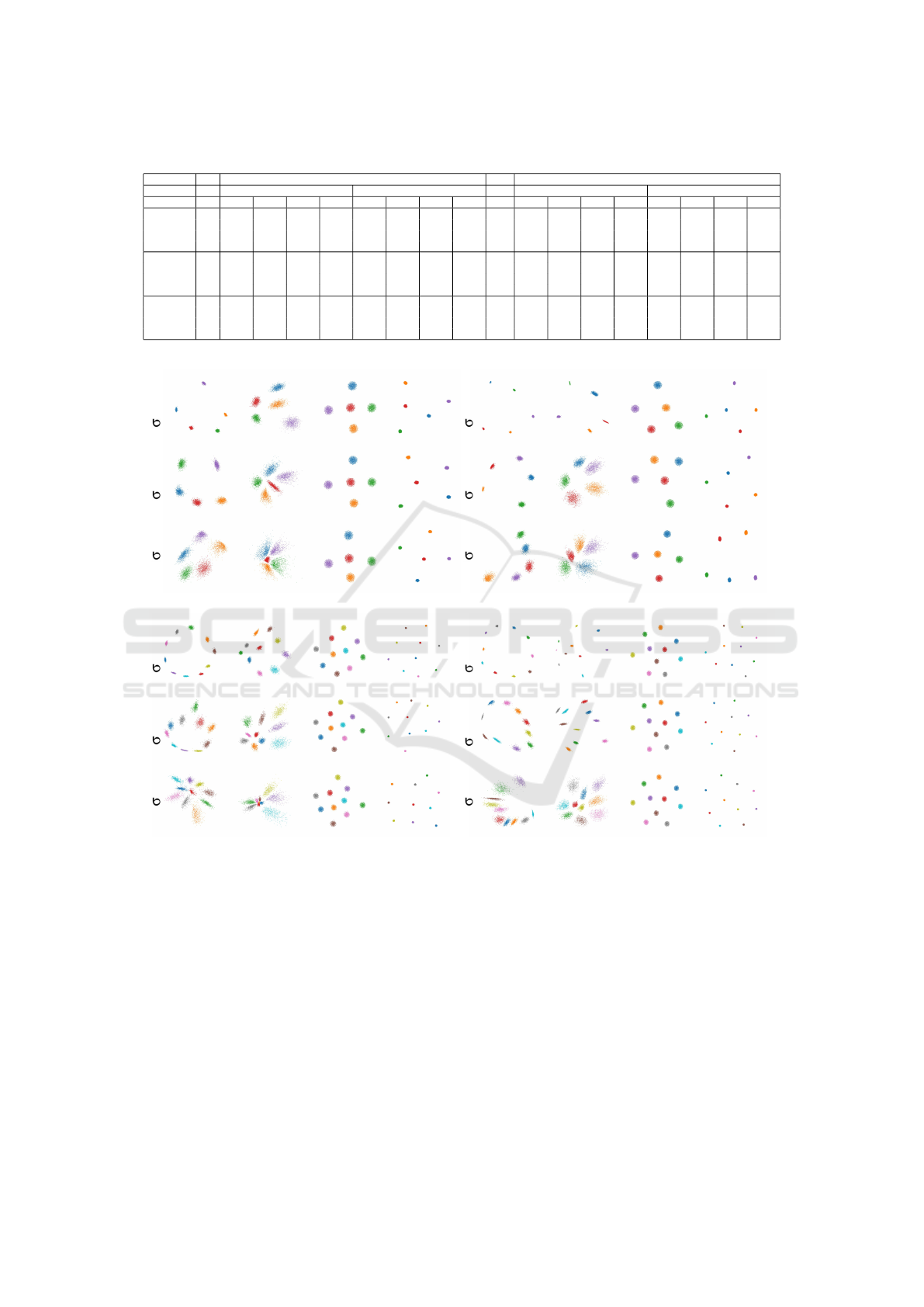
Table 3: Quality measurements for the synthetic blobs experiment with 100 and 700 dimensions, 5 and 10 cluster centers.
100 dimensions 700 dimensions
5 clusters 10 clusters 5 clusters 10 clusters
Algorithm σ T C R N T C R N σ T C R N T C R N
AE
1.3
0.923 0.938 0.547 1.000 0.958 0.963 0.692 1.000
1.6
0.909 0.914 0.739 1.000 0.953 0.955 0.254 1.000
t-SNE 0.937 0.955 0.818 1.000 0.967 0.977 0.192 1.000 0.917 0.951 0.362 1.000 0.960 0.976 0.346 1.000
UMAP 0.921 0.949 0.868 1.000 0.957 0.970 0.721 1.000 0.906 0.933 0.878 1.000 0.954 0.965 0.471 1.000
SSNP-KM 0.910 0.919 0.687 1.000 0.956 0.959 0.602 1.000 0.904 0.908 0.568 1.000 0.953 0.955 0.399 1.000
AE
3.9
0.919 0.926 0.750 1.000 0.959 0.963 0.484 1.000
4.8
0.910 0.914 0.615 1.000 0.953 0.954 0.354 1.000
t-SNE 0.931 0.953 0.707 1.000 0.966 0.978 0.227 1.000 0.914 0.950 0.608 1.000 0.960 0.977 0.331 1.000
UMAP 0.911 0.940 0.741 1.000 0.956 0.969 0.537 1.000 0.906 0.931 0.697 1.000 0.954 0.965 0.390 1.000
SSNP-KM 0.910 0.918 0.622 1.000 0.955 0.958 0.549 1.000 0.905 0.907 0.612 1.000 0.953 0.954 0.296 1.000
AE
9.1
0.905 0.901 0.569 1.000 0.938 0.945 0.328 0.999
11.2
0.911 0.906 0.600 1.000 0.955 0.954 0.382 1.000
t-SNE 0.913 0.951 0.533 1.000 0.948 0.974 0.254 1.000 0.914 0.950 0.492 1.000 0.959 0.977 0.296 1.000
UMAP 0.888 0.939 0.535 1.000 0.929 0.966 0.342 1.000 0.905 0.931 0.557 1.000 0.953 0.965 0.336 1.000
SSNP-KM 0.888 0.917 0.595 0.998 0.927 0.952 0.437 0.995 0.904 0.906 0.557 1.000 0.950 0.945 0.314 0.998
700 dimensions, 5 clusters
=11.2 =4.8 =1.6
SSNP (Km) Autoencoder t-SNE UMAP
700 dimensions, 10 clusters
SSNP (Km) Autoencoder t-SNE UMAP
100 dimensions, 5 clusters
=9.1 =3.9 =1.3
SSNP (Km) Autoencoder t-SNE UMAP
100 dimensions, 10 clusters
SSNP (Km) Autoencoder t-SNE UMAP
=9.1 =3.9 =1.3
=11.2 =4.8 =1.6
Figure 4: Projection of synthetic blobs datasets with SSNP(Km) and other techniques, with different number of dimensions
and clusters. In each quadrant, rows show datasets having increasing standard deviation σ.
very close to the ones created by the technique it is
trying to mimic, typically t-SNE– see e.g. (Espadoto
et al., 2020).
Table 3 shows the quality measurements for this
experiment for the datasets using 5 and 10 cluster
centers. We see that SSNP performs very similarly
quality-wise to AE, t-SNE, and UMAP. We will bring
more insight to this comparison in Section 4.2, which
studies more challenging, real-world, datasets.
4.2 Quality: Real-world Datasets
Figure 5 shows in the first three columns the projec-
tion of real-world datasets by SSNP using pseudo-
labels assigned by K-means and Agglomerative Clus-
tering, alongside the projection created by an autoen-
coder. The next three columns show the same datasets
projected by t-SNE, UMAP, and SSNP using ground-
truth labels. Again, we omit the plots and measure-
ments for NNP, since they are very close to the ones
created by t-SNE and UMAP.
IVAPP 2021 - 12th International Conference on Information Visualization Theory and Applications
32
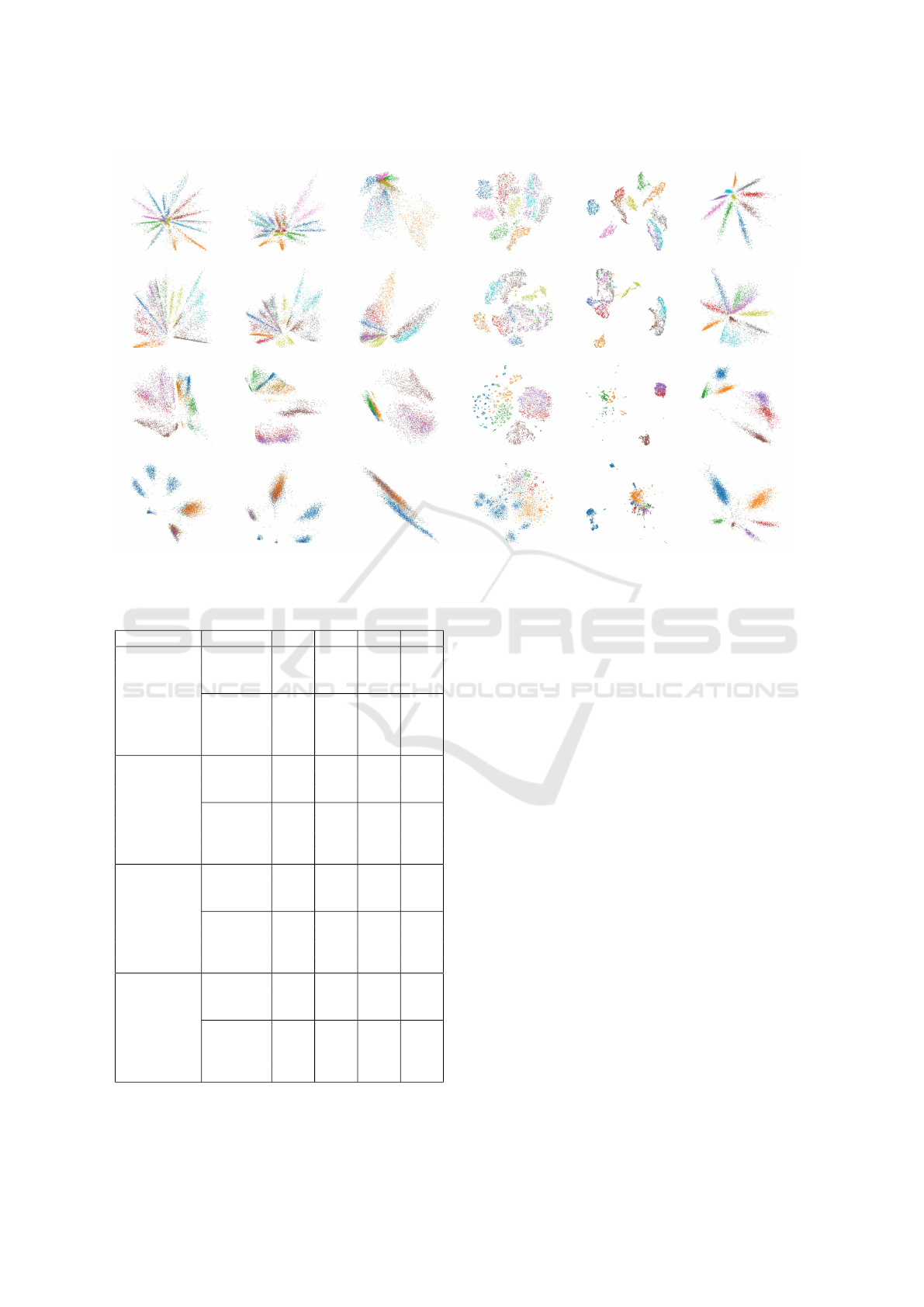
SSNP (Km) SSNP (Agg) Autoencoder t-SNE UMAP SSNP (GT)
Reuters HAR FashionMNIST MNIST
Figure 5: Projection of real-world datasets with SSNP and other techniques. Left to right: SSNP using K-means, SSNP using
Agglomerative clustering, Autoencoder, t-SNE, UMAP, and SSNP using ground truth labels.
Table 4: Quality measurements for the real-world datasets.
Dataset Method T C R NH
MNIST
SSNP(Km) 0.882 0.903 0.264 0.767
SSNP(Agg) 0.859 0.925 0.262 0.800
AE 0.887 0.920 0.009 0.726
SSNP(GT) 0.774 0.920 0.398 0.986
NNP 0.948 0.969 0.397 0.891
t-SNE 0.985 0.972 0.412 0.944
UMAP 0.958 0.974 0.389 0.913
FashionMNIST
SSNP(Km) 0.958 0.982 0.757 0.739
SSNP(Agg) 0.950 0.978 0.707 0.753
AE 0.961 0.977 0.538 0.725
SSNP(GT) 0.863 0.944 0.466 0.884
NNP 0.963 0.986 0.679 0.765
t-SNE 0.990 0.987 0.664 0.843
UMAP 0.982 0.988 0.633 0.805
HAR
SSNP(Km) 0.932 0.969 0.761 0.811
SSNP(Agg) 0.926 0.964 0.724 0.846
AE 0.937 0.970 0.805 0.786
SSNP(GT) 0.876 0.946 0.746 0.985
NNP 0.961 0.984 0.592 0.903
t-SNE 0.992 0.985 0.578 0.969
UMAP 0.980 0.989 0.737 0.933
Reuters
SSNP(Km) 0.794 0.859 0.605 0.738
SSNP(Agg) 0.771 0.824 0.507 0.736
AE 0.747 0.731 0.420 0.685
SSNP(GT) 0.720 0.810 0.426 0.977
NNP 0.904 0.957 0.594 0.860
t-SNE 0.955 0.959 0.588 0.887
UMAP 0.930 0.963 0.674 0.884
Figure 5 shows that SSNP with pseudo-labels
shows better cluster separation than Autoencoders,
and, for more challenging datasets, such as HAR and
Reuters, SSNP with ground-truth labels looks better
than t-SNE and UMAP. SSNP and Autoencoder were
trained for 10 epochs in all cases. SSNP used twice
the number of classes as the target number of clus-
ters for the clustering algorithms used for pseudo-
labeling. We see also that SSNP creates elongated
clusters, in a star-like pattern. We believe this is due to
the fact that one of the targets of the network is a clas-
sifier, which is trained to partition the space based on
the data. This results in placing samples that are near
a decision boundary between classes closer to the cen-
ter of the star pattern; samples that are far away from a
decision boundary are placed near the tips of the star,
according to its class.
Table 4 shows the quality measurement for this ex-
periment. We see that SSNP with pseudo-labels con-
sistently shows better cluster separation than Autoen-
coders, as measured by the NH, as well as better dis-
tance correlation, as measured by R. For the harder
HAR and Reuters datasets, SSNP with ground-truth
labels shows NH results that are competitive and even
better than the ones for t-SNE and UMAP. For the
T and C metrics, SSNP outperforms again Autoen-
coders in most cases; for FashionMNIST and HAR,
SSNP yields T and C values close to the ones for
NNP, t-SNE, and UMAP.
Self-supervised Dimensionality Reduction with Neural Networks and Pseudo-labeling
33
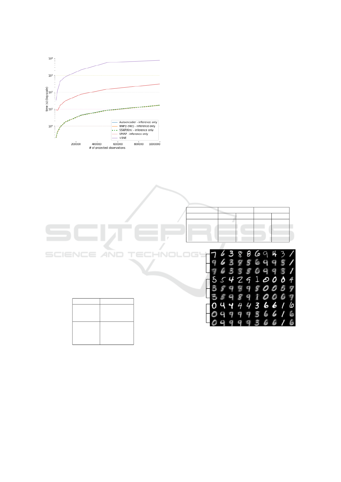
Figure 6: Inference time for SSNP and other techniques.
All techniques trained with 10K samples from the MNIST
dataset. Inference done on MNIST upsampled up to 1M
samples.
4.3 Computational Scalability
Table 5 shows the time required to set up SSNP and
other projection techniques. For SSNP, this means
training the network. For t-SNE, this means actual
projection of the data, since this technique is non-
parametric. All SSNP variants take far under a minute
to set up, with SSNP(GT) being the fastest, as it does
not need the clustering step. Of the pseudo-labeling
varieties, SSNP(Km) is the fastest. We used 10K
training samples, which is on the conservative side.
In practice, we get good results (quality-wise) with as
few as 1K samples.
Table 5: Set-Up time for different methods, using 10K train-
ing samples, MNIST dataset. All SSNP variants and Au-
toencoders were trained for 10 epochs. t-SNE is here for
reference only, since it is a non-parametric technique.
Method Training time (s)
SSNP(GT) 6.029
SSNP(Km) 20.478
SSNP(Agg) 31.954
Autoencoder 3.734
UMAP 25.143
t-SNE 33.620
NNP(t-SNE) 51.181
Figure 6 shows the time needed to project up to
1M samples using SSNP and the other techniques.
Being GPU-accelerated neural networks, SSNP, Au-
toencoders and NNP perform very fast, all being able
to project up to 1M samples in a few seconds – an
order of magnitude faster than UMAP, and over three
orders of magnitude faster than t-SNE.
4.4 Inverse Projection
Figure 7 shows a set of digits from the MNIST
dataset – both the actual images x and the ones ob-
tained by inverse projection P
−1
(P(x)). We see that
SSNP(Km) yields results very similar to Autoen-
coders, so SSNP’s dual-optimization target succeeds
in learning a good inverse mapping based on the di-
rect mapping given by the pseudo-labels (Section 3).
Table 6 strengthens this insight by showing the val-
ues for Mean Squared Error between original and
inversely-projected data for SSNP(Km) and Autoen-
coder, which, again, are very similar. Furthermore,
the SSNP MSE errors are of the same order of mag-
nitude – that is, small – as those obtained by the re-
cent NNInv technique and the older iLAMP (Amorim
et al., 2012) one – compare Table 6 with Figure
2 in (Espadoto et al., 2019b), not included here for
space reasons.
Table 6: Inverse projection Mean Square Error (MSE) for
SSNP(Km) and Autoencoder, trained with 5K samples,
tested with 1K samples.
SSNP(Km) Autoencoder
Dataset Train Test Train Test
MNIST 0.0474 0.0480 0.0424 0.0440
FashionMNIST 0.0309 0.0326 0.0291 0.0305
HAR 0.0072 0.0074 0.0066 0.0067
Reuters 0.0002 0.0002 0.0002 0.0002
Original
Autoencoder
SSNP(Km)
Original
Autoencoder
SSNP(Km)
Original
Autoencoder
SSNP(Km)
Figure 7: Sample images from MNIST inversely projected
by SSNP and Autoencoder, both trained with 10 epochs and
5K samples. Bright images show the original data.
4.5 Data Clustering
Table 7 shows how SSNP performs when doing clas-
sification or clustering, which corresponds respec-
tively to its usage of pseudo-labels or ground-truth
labels. We see that SSNP generates good results in
both cases when compared to the ground-truth labels
and, respectively, the underlying clustering algorithm.
We stress that this is a side result of SSNP. While one
IVAPP 2021 - 12th International Conference on Information Visualization Theory and Applications
34

gets this for free, SSNP only mimics the underlying
clustering algorithm that it learns, rather than doing
clustering from scratch.
Table 7: Classification/clustering accuracy of SSNP when
compared to ground truth (GT) and clustering labels (Km),
trained with 5K observations, test with 1K observations.
SSNP(GT) SSNP(Km)
Dataset Train Test Train Test
MNIST 0.984 0.942 0.947 0.817
FashionMNIST 0.866 0.815 0.902 0.831
HAR 0.974 0.974 0.931 0.919
Reuters 0.974 0.837 0.998 0.948
4.6 Implementation Details
All experiments discussed above were run on a 4-
core Intel Xeon E3-1240 v6 at 3.7 GHz with 64 GB
RAM and an NVidia GeForce GTX 1070 GPU with
8 GB VRAM. Table 8 lists all open-source software
libraries used to build SSNP and the other tested tech-
niques. Our neural network implementation lever-
ages the GPU power by using the Keras framework.
The t-SNE implementation used is a parallel version
of Barnes-Hut t-SNE (Ulyanov, 2016; Maaten, 2013),
run on all four available CPU cores for all tests. The
UMAP reference implementation is not parallel, but
is quite fast (compared to t-SNE) and well-optimized.
Our implementation, plus all code used in this ex-
periment, are publicly available at https://github.com/
mespadoto/ssnp.
Table 8: Software used for the evaluation.
Technique Software used publicly available at
SSNP (our technique) keras.io (TensorFlow backend)
Autoencoder
t-SNE github.com/DmitryUlyanov/Multicore-t-SNE
UMAP github.com/lmcinnes/umap
K-means scikit-learn.org
Agglomerative Clustering
5 DISCUSSION
We discuss next how SSNP performs with respect to
the seven criteria laid out in Section 1.
Quality (C1). As shown in Figures 4 and 5, SSNP
provides better cluster separation than Autoencoders,
as measured by the selected metrics (Tables 3 and
4). The choice of clustering algorithm does not seem
to be a key factor, with K-means and Agglomer-
ative clustering yielding similar results for all metrics;
Scalability (C2). SSNP, while not as fast to train as
standard Autoencoders, is still very fast, with most of
the training time being used by clustering – visible
by the fact that SSNP(GT)’s training time is close
to Autoencoder’s one. In our experiments, K-means
seems to be faster than Agglomerative clustering,
being thus more suitable when training SSNP with
very large datasets. Inference time for SSNP is
very close to Autoencoders and NNP, and much
faster than UMAP (let alone t-SNE), which shows
SSNP’s suitability to cases where one needs to project
large amounts of data, such as streaming applications;
Ease of Use (C3). SSNP yielded good projection
results with little training (10 epochs), little training
data (5K samples) and a simple heuristic of setting
the number of clusters for the clustering step to
twice the number of expected clusters in the data.
Other clustering techniques which do not require
setting the number of clusters can be used, such as
DBSCAN (Ester et al., 1996) and Affinity Propaga-
tion (Frey and Dueck, 2007), making SSNP usage
even simpler. We see this experiments as part of
future work;
Genericity (C4). We show results for SSNP with dif-
ferent types of high-dimensional data, namely tabular
(HAR), images (MNIST, FashionMNIST), and text
(Reuters). We believe this shows the versatility of the
method;
Stability and Out-of-Sample Support (C5). All
measurements we show for SSNP are based on
inference, i.e., we pass the data through the trained
network to compute them. This is evidence of the
out-of-sample capability, which allows one to project
new data without recomputing the projection, as is
the case for t-SNE and other non-parametric methods;
Inverse Mapping (C6). SSNP shows inverse map-
ping results which are, quality-wise, very similar
to results from Autoencoders, NNInv and iLAMP,
which is evidence of SSNP’s inverse mapping abili-
ties;
Clustering (C7). SSNP is able to mimic the behav-
ior of the clustering algorithm used as its input, as
a byproduct of the training with labels. We show that
SSNP produces competitive results when compared to
pseudo- or ground truth labels. Although SSNP is not
a clustering algorithm, it provides this for free (with
no additional execution cost), which can be useful in
cases where one wants to do both clustering and DR.
In addition to the good performance shown for the
aforementioned criteria, a key strength of SSNP is its
ability of performing all the operations described in
Section 4 after a single training phase, which saves
effort and time in cases where all or a subset of
Self-supervised Dimensionality Reduction with Neural Networks and Pseudo-labeling
35

those results (e.g., direct projection, inverse projec-
tion, clustering) are needed.
6 CONCLUSION
We presented a new dimensionality reduction tech-
nique called SSNP. Through several experiments,
we showed that SSNP creates projections of high-
dimensional data that obtain a better visual clus-
ter separation than autoencoders, the technique that
SSNP is closest to, and have similar (albeit slightly
lower) quality to those obtained by state-of-the-art
methods. SSNP is, to our knowledge, the only tech-
nique that jointly addresses all characteristics listed
in Section 1 of this paper, namely producing projec-
tions that exhibit a good visual separation of simi-
lar samples, handling datasets of millions of elements
in seconds, being easy to use (no complex parame-
ters to set), handling generically any type of high-
dimensional data, providing out-of-sample support,
and providing an inverse projection function.
One low-hanging fruit is to study SSNP in con-
junction with more advanced clustering algorithms
than the K-means and agglomerative clustering used
in this paper, yielding potentially even better visual
cluster separation. A more ambitious, but realizable,
goal is to have SSNP learn its pseudo-labeling dur-
ing training and therefore remove the need for using a
separate clustering algorithm. We plan to explore this
directions in future work.
ACKNOWLEDGMENTS
This study was financed in part by FAPESP
(2015/22308-2 and 2017/25835-9) and the
Coordenac¸
˜
ao de Aperfeic¸oamento de Pessoal de
N
´
ıvel Superior - Brasil (CAPES) - Finance Code 001.
REFERENCES
Amorim, E., Brazil, E. V., Daniels, J., Joia, P., Nonato,
L. G., and Sousa, M. C. (2012). iLAMP: Exploring
high-dimensional spacing through backward multidi-
mensional projection. In Proc. IEEE VAST, pages 53–
62.
Anguita, D., Ghio, A., Oneto, L., Parra, X., and Reyes-
Ortiz, J. L. (2012). Human activity recognition
on smartphones using a multiclass hardware-friendly
support vector machine. In Proc. Intl. Workshop on
Ambient Assisted Living, pages 216–223. Springer.
Becker, M., Lippel, J., Stuhlsatz, A., and Zielke, T. (2020).
Robust dimensionality reduction for data visualiza-
tion with deep neural networks. Graphical Models,
108:101060.
Becker, R., Cleveland, W., and Shyu, M. (1996). The visual
design and control of trellis display. Journal of Com-
putational and Graphical Statistics, 5(2):123–155.
Chan, D., Rao, R., Huang, F., and Canny, J. (2018). T-SNE-
CUDA: GPU-accelerated t-SNE and its applications
to modern data. In Proc. SBAC-PAD, pages 330–338.
Cunningham, J. and Ghahramani, Z. (2015). Linear dimen-
sionality reduction: Survey, insights, and generaliza-
tions. JMLR, 16:2859–2900.
Donoho, D. L. and Grimes, C. (2003). Hessian eigen-
maps: Locally linear embedding techniques for high-
dimensional data. Proc Natl Acad Sci, 100(10):5591–
5596.
Engel, D., Hattenberger, L., and Hamann, B. (2012). A
survey of dimension reduction methods for high-
dimensional data analysis and visualization. In Proc.
IRTG Workshop, volume 27, pages 135–149. Schloss
Dagstuhl.
Espadoto, M., Hirata, N., and Telea, A. (2020). Deep learn-
ing multidimensional projections. J. Information Vi-
sualization. doi.org/10.1177/1473871620909485.
Espadoto, M., Martins, R. M., Kerren, A., Hirata, N. S., and
Telea, A. C. (2019a). Towards a quantitative survey of
dimension reduction techniques. IEEE TVCG. Pub-
lisher: IEEE.
Espadoto, M., Rodrigues, F. C. M., Hirata, N. S. T., Hi-
rata Jr., R., and Telea, A. C. (2019b). Deep learning in-
verse multidimensional projections. In Proc. EuroVA.
Eurographics.
Ester, M., Kriegel, H.-P., Sander, J., Xu, X., et al. (1996).
A density-based algorithm for discovering clusters in
large spatial databases with noise. In Proc. KDD,
pages 226–231.
Fisher, R. A. (1936). The use of multiple measurements in
taxonomic problems. Annals of eugenics, 7(2):179–
188.
Frey, B. J. and Dueck, D. (2007). Clustering by
passing messages between data points. Science,
315(5814):972–976. Publisher: AAAS.
Hinton, G. E. and Salakhutdinov, R. R. (2006). Reducing
the dimensionality of data with neural networks. Sci-
ence, 313(5786):504–507. Publisher: AAAS.
Hoffman, P. and Grinstein, G. (2002). A survey of visualiza-
tions for high-dimensional data mining. Information
Visualization in Data Mining and Knowledge Discov-
ery, 104:47–82. Publisher: Morgan Kaufmann.
Inselberg, A. and Dimsdale, B. (1990). Parallel coordinates:
A tool for visualizing multi-dimensional geometry. In
Proc. IEEE Visualization, pages 361–378.
Joia, P., Coimbra, D., Cuminato, J. A., Paulovich, F. V., and
Nonato, L. G. (2011). Local affine multidimensional
projection. IEEE TVCG, 17(12):2563–2571.
Jolliffe, I. T. (1986). Principal component analysis and fac-
tor analysis. In Principal Component Analysis, pages
115–128. Springer.
IVAPP 2021 - 12th International Conference on Information Visualization Theory and Applications
36

Kaufman, L. and Rousseeuw, P. (2005). Finding Groups in
Data: An Introduction to Cluster Analysis. Wiley.
Kehrer, J. and Hauser, H. (2013). Visualization and vi-
sual analysis of multifaceted scientific data: A survey.
IEEE TVCG, 19(3):495–513.
Kingma, D. P. and Welling, M. (2013). Auto-encoding
variational bayes. CoRR, abs/1312.6114. eprint:
1312.6114.
Kohonen, T. (1997). Self-organizing Maps. Springer.
LeCun, Y. and Cortes, C. (2010). MNIST handwritten digits
dataset. http://yann.lecun.com/exdb/mnist.
Liu, S., Maljovec, D., Wang, B., Bremer, P.-T., and
Pascucci, V. (2015). Visualizing high-dimensional
data: Advances in the past decade. IEEE TVCG,
23(3):1249–1268.
Lloyd, S. (1982). Least squares quantization in PCM. IEEE
Trans Inf Theor, 28(2):129–137.
Maaten, L. v. d. (2013). Barnes-hut-SNE. arXiv preprint
arXiv:1301.3342.
Maaten, L. v. d. (2014). Accelerating t-SNE using tree-
based algorithms. JMLR, 15:3221–3245.
Maaten, L. v. d. and Hinton, G. (2008). Visualizing data
using t-SNE. JMLR, 9:2579–2605.
Maaten, L. v. d. and Postma, E. (2009). Dimensionality
reduction: A comparative review. Technical report,
Tilburg University, Netherlands.
Martins, R. M., Minghim, R., Telea, A. C., and others
(2015). Explaining neighborhood preservation for
multidimensional projections. In CGVC, pages 7–14.
McInnes, L. and Healy, J. (2018). UMAP: Uniform man-
ifold approximation and projection for dimension re-
duction. arXiv:1802.03426v1 [stat.ML].
Nonato, L. and Aupetit, M. (2018). Multidimensional
projection for visual analytics: Linking techniques
with distortions, tasks, and layout enrichment. IEEE
TVCG.
Paulovich, F. V. and Minghim, R. (2006). Text map ex-
plorer: a tool to create and explore document maps.
In Proc. Intl. Conference on Information Visualisation
(IV), pages 245–251. IEEE.
Paulovich, F. V., Nonato, L. G., Minghim, R., and Lev-
kowitz, H. (2008). Least square projection: A fast
high-precision multidimensional projection technique
and its application to document mapping. IEEE
TVCG, 14(3):564–575.
Pezzotti, N., H
¨
ollt, T., Lelieveldt, B., Eisemann, E., and
Vilanova, A. (2016). Hierarchical stochastic neighbor
embedding. Computer Graphics Forum, 35(3):21–30.
Pezzotti, N., Lelieveldt, B., Maaten, L. v. d., H
¨
ollt, T., Eise-
mann, E., and Vilanova, A. (2017). Approximated and
user steerable t-SNE for progressive visual analytics.
IEEE TVCG, 23:1739–1752.
Pezzotti, N., Thijssen, J., Mordvintsev, A., Hollt, T., Lew,
B. v., Lelieveldt, B., Eisemann, E., and Vilanova, A.
(2020). GPGPU linear complexity t-SNE optimiza-
tion. IEEE TVCG, 26(1):1172–1181.
Rao, R. and Card, S. K. (1994). The table lens: Merging
graphical and symbolic representations in an interac-
tive focus+context visualization for tabular informa-
tion. In Proc. ACM SIGCHI, pages 318–322.
Roweis, S. T. and Saul, L. L. K. (2000). Nonlinear di-
mensionality reduction by locally linear embedding.
Science, 290(5500):2323–2326. Publisher: American
Association for the Advancement of Science.
Salton, G. and McGill, M. J. (1986). Introduction to modern
information retrieval. McGraw-Hill.
Sorzano, C., Vargas, J., and Pascual-Montano, A. (2014).
A survey of dimensionality reduction techniques.
arXiv:1403.2877 [stat.ML].
Telea, A. C. (2006). Combining extended table lens and
treemap techniques for visualizing tabular data. In
Proc. EuroVis, pages 120–127.
Tenenbaum, J. B., Silva, V. D., and Langford, J. C. (2000).
A global geometric framework for nonlinear dimen-
sionality reduction. Science, 290(5500):2319–2323.
Thoma, M. (2017). The Reuters dataset.
Torgerson, W. S. (1958). Theory and Methods of Scaling.
Wiley.
Ulyanov, D. (2016). Multicore-TSNE.
Venna, J. and Kaski, S. (2006). Visualizing gene interaction
graphs with local multidimensional scaling. In Proc.
ESANN, pages 557–562.
Wattenberg, M. (2016). How to use t-SNE effectively. https:
//distill.pub/2016/misread-tsne.
Xiao, H., Rasul, K., and Vollgraf, R. (2017). Fashion-
MNIST: A novel image dataset for benchmarking ma-
chine learning algorithms. arXiv:1708.07747.
Xie, H., Li, J., and Xue, H. (2017). A survey of dimen-
sionality reduction techniques based on random pro-
jection. arXiv:1706.04371 [cs.LG].
Yates, A., Webb, A., Sharpnack, M., Chamberlin, H.,
Huang, K., and Machiraju, R. (2014). Visualizing
multidimensional data with glyph SPLOMs. Com-
puter Graphics Forum, 33(3):301–310.
Zhang, Z. and Wang, J. (2007). MLLE: Modified lo-
cally linear embedding using multiple weights. In
Advances in Neural Information Processing Systems
(NIPS), pages 1593–1600.
Zhang, Z. and Zha, H. (2004). Principal manifolds and
nonlinear dimensionality reduction via tangent space
alignment. SIAM Journal on Scientific Computing,
26(1):313–338.
Self-supervised Dimensionality Reduction with Neural Networks and Pseudo-labeling
37
