
Indextron
Alexei Mikhailov
a
and Mikhail Karavay
b
Institute of Control Problems, Russian Acad. of Sciences, Profsoyuznaya Street, 65, Moscow, Russia
Keywords: Pattern Recognition, Machine Learning, Neural Networks, Inverse Sets, Inverse Patterns, Multidimensional
Indexing.
Abstract: How to do pattern recognition without artificial neural networks, Bayesian classifiers, vector support
machines and other mechanisms that are widely used for machine learning? The problem with pattern
recognition machines is time and energy demanding training because lots of coefficients need to be worked
out. The paper introduces an indexing model that performs training by memorizing inverse patterns mostly
avoiding any calculations. The computational experiments indicate the potential of the indexing model for
artificial intelligence applications and, possibly, its relevance to neurobiological studies as well.
a
https://orcid.org/0000-0001-8601-4101
b
https://orcid.org/0000-0002-9343-366X
1 INTRODUCTION
Typically, pattern classification amounts to
assigning a given pattern
x to a class
k
out of K
available classes. For this,
K class probabilities
12
( ), ( ),..., ( )
K
pp pxx x
need to be calculated, after
which the pattern
x is assigned to the class
k
with a
maximum probability
()
k
p x
(Theodoridis, S. and
Koutroumbas, K. , 2006). This paper avoids a
discussion of classification devices, directly
proceeding to finding class probabilities by a pattern
inversion. Not only such approach cuts down on
training costs, it might also be useful in studying
biological networks, where details of intricate
connectivity of neuronal patterns may not need to be
unraveled. Then, for a given set of patterns, results
of computational experiments can be compared to
that of physical experiments.
For example, Tsunoda et al. (2001) demonstrated
that “objects are represented in macaque
inferotemporal (IT) cortex by combinations of
feature columns”. Figure 1 shows the images that
were taken by Tsunoda et al. (2001) with a camera
attached above a monkey’s IT-region, where a piece
of skull was removed. The anaesthetized monkey’s
IT-region responded to three cat-doll pictures, which
were shown, in turn, with active spots marked by
red, blue and green circles, correspondingly. The
active spots appear on the IT-cortical map because
the neurons under these spots exert increased blood
flow, which is registered by an infrared camera. A
clear set-theoretical inclusion pattern was observed,
in which blue circles make a subset of red circles
and green circles make a subset of blue circles.
This paper describes an experiment, where
similar real cat pictures were shown to an indexing
model referred to as the indextron. The outcomes are
presented in (Figure1, IM) and annotated in the
section Results, points 1.
Also, a comparative performance of the
indextron versus artificial neural networks and
decision functions was tested against benchmark
datasets (see the section Results, points 2 - 3).
Comments are provided in the section 3. The
indextron is considered in details in the Section 4.
2 RESULTS
1) A set-theoretical inclusion pattern, which is
similar to that in Figure 1, IT, was observed in the
memory of the indextron (Figure 1, IM). For that,
this model was shown, in turn, complete and partial
real cat images D, E, F retrieved from (Les Chats,
2010).
Mikhailov, A. and Karavay, M.
Indextron.
DOI: 10.5220/0010180301430149
In Proceedings of the 10th International Conference on Pattern Recognition Applications and Methods (ICPRAM 2021), pages 143-149
ISBN: 978-989-758-486-2
Copyright
c
2021 by SCITEPRESS – Science and Technology Publications, Lda. All rights reserved
143
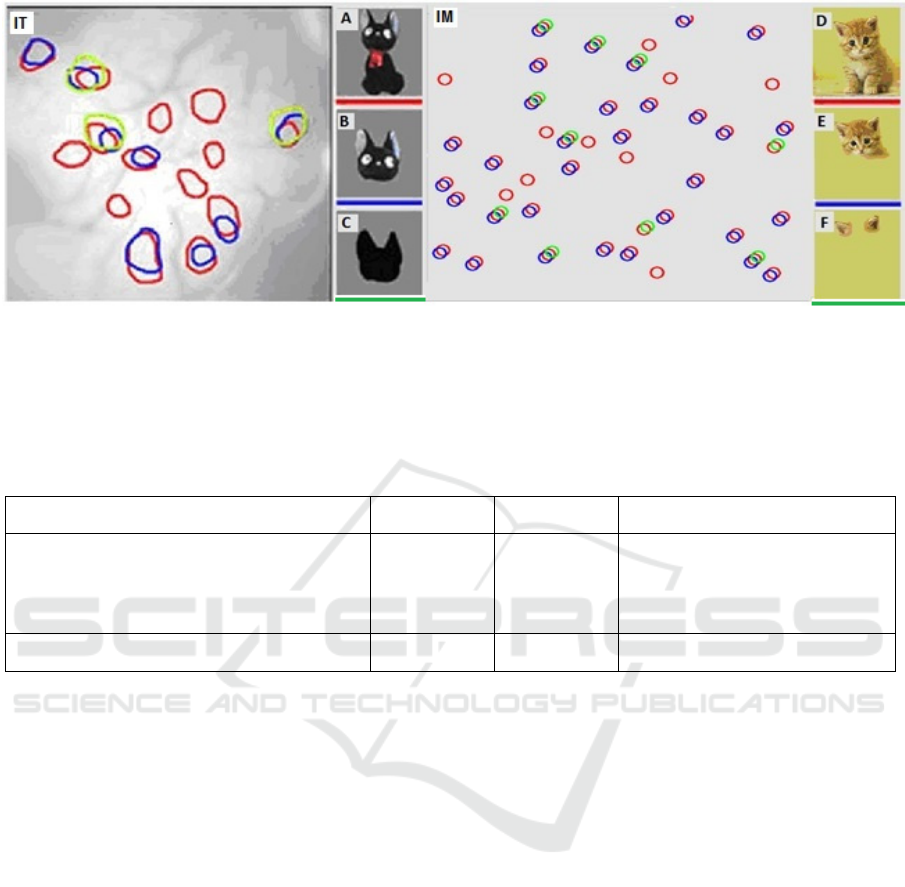
Figure 1: Activity in IT-region of a monkey and in the indextron memory (IM): (IT) The encircled areas were activated in
IT-region of a monkey by cat-doll pictures. (A) Full cat-doll picture activated read areas. (B) Head cat-doll picture activated
blue areas. (C) Head contour cat-doll picture activated green areas. (IM) Activity elicited in the model (a part of indextron
memory is shown). (D) Full real cat picture activated read circles in IM. (E) Head picture activated blue areas in IM.
(F) Ears activated green areas in IM. A clear set-theoretical inclusion pattern, where green circles are subsets of blue circles
that are, in turn, subsets of red circles, is observed in both the IT-region and the model.
Table 1: Neural network versus indexing classifier.
Classifier Accuracy (%) Training (sec) Hardware & Libraries
4 layer neural network *)
Layers: Flatten, Dropout,
Dense (256 neurons, ReLu activation function),
Dense (10 neurons, softmax)
85.3 900 AMD Ryzen 5 3600, Python,
Nvidia GeForce GTX 1660 Super,
TensorFlow, Keras, cuDNN
Indextron 82.87 16 AMD Ryzen 5 3600, Python
*) For feature extraction, the convolutional neural network VGG16 from the web-site KERAS (2019) had been pre-trained
on the ImageNet database (2016). Next, VGG16 was trained on 50000 grey level 32x32 images (10 categories) from the
CIFAR-10 dataset providing 512 features per image. Finally, 512 x 50000 features were used for training both a 4-layer
neural network and the indextron. For testing, 10000 images (512 x 10000 features) from the above dataset were classified
using both the 4- layer neural network and the indextron.
2) CIFAR – 10 dataset (Krizhevsky et al, 2009) was
used for testing the indextron against artificial neural
networks. It was shown that the indextron reduced
the training time by the factor of 50 in comparison to
a 4-layer neural network (ref. to Table 1).
3) The indextron’s performance against decision
functions was tested with the CoverType dataset
(Chang D., Canny J., 2014). It was shown that the
indextron algorithm running on a 1.6 MHz CPU
outperformed by a factor of 2 a much more powerful
4-GPU NVidia platform (ref. to Table 2).
3 DISCUSSION
1) The structure of the indextron algorithm
resembles that of a back-of-the-book index. If the
observed similarity of responses between the
indextron and a biological cortical region is not a
coincidence, then it might be possible to suggest that
cortical regions work similar to indexing systems,
where input features serve as keywords activating
outcomes with little or no arithmetic.
2) The fact that at a competitive 85% accuracy, a
mundane 2-core CPU outperforms in terms of
throughput a much more powerful 4-GPU, 8-core
CPU
platform can be explained by the simplicity of
the indextron algorithm, which does not involve any
floating-point operation, multiplications and
adjustable coefficients.
3) Figure 1, IT, shows only a 10% sub-area of active
model area, - the sub-area, which fits the image.
Nonetheless, the inclusion relationship holds
throughout the entire area.
ICPRAM 2021 - 10th International Conference on Pattern Recognition Applications and Methods
144

Table 2: Time and accuracy of classifiers at train / test samples 290506 / 290506 Cover Type dataset division.
Platform Method Training Time (sec) Accuracy %
4GPU (NVidia GT X-690 64GB RAM
8-core CPU at 2.2 GHz
SkiKit 138.17 87.7
CudaTree 30.47 96.0
BiDMachRF 67.27 71.0
Dual-core CPU at 1.6MHz 3GB RAM Indextron 16* 90
4) Experiments with the indextron suggest that two
monkeys looking at the same pictures may elicit
different active spot arrangements in their IT-region
as they most probably learnt their visual experiences
in different circumstances.
4 MATERIALS AND METHODS
4.1 Feature Extraction
Sets of local features were used to represent real
cat’s images from (Les Chats, 2010) (see Figure 1,
(D, E, F)). Each color image was converted to a grey
level image that was subject to edge detection
followed by thinning out a list of edge points. For
each remaining edge point, a histogram of distances
from a current point to its 20 nearest neighbors was
created to represent this point’s vicinity by a feature
vector
12
( , ,..., )
N
x
xx=x
Next, this vicinity was
classified in an unsupervised fashion by the
indextron model, where each active vicinity was
represented by a cell on a two-dimensional memory
plane. Since there does not exist a one-to-one
mapping between an
N -dimensional ( 2N > )
space and a two-dimensional plane, the active cells
were randomly placed on the plane on a first-come-
first-occupy basis (shown by circles on Figure. 1,
(IT)). Colors of the circles represent 2
nd
level classes
(body, head, and ears), where a 2
nd
level class was
assigned a red, blue or green color, respectively.
2
nd
level classifier takes as its input a histograms of
1
st
level classes, i.e., a histograms of vicinity classes.
4.2 Pattern Classification
This paper introduces an indexing classifier referred
to as the indextron. The indextron comprises a
number of identical levels. Each level takes in as its
input either a feature vector or a feature set and
returns an index that represents the input’s class.
Once a set of indexes has been accumulated, a
histogram of indexes can be used as an input for the
next level, which returns its output index that
represents a meta-class of first level inputs. And so
on “up to infinity”. A single level classification
problem can be summarized in strict mathematical
terms as follows.
Let all variables be integers and
K pattern
classes be represented by a collection of
K vectors
,1 , ,
,..., ,..., , 1,2,...,
kknkN
K
xxxk=
(1)
in N-dimensional space, such that all vector
components are restricted as
,
0
kn
x
X£<
. It is
also assumed that the Chebyshev distance between
any two vectors
,kj
is greater than R, that is, any
two vectors differ in at least one component
,,
, : | |
kn jn
kj n x x R"$ - >
Problem: Given an unknown vector
( ), 1,2,...,
x
nn N=
, find its class, that is, find
the vector k from the given collection, such that the
Chebyshev distance between these two vectors is
less than R
,
| ( ) |
kn
nxn x R"-£
Solution: Consider the indexed sets
,
{}
x
n
k
defined
as
,,
{} { : | () | }
0 , 1,2,...,
xn kn
kkxnxR
xXn N
=-£
£< =
(2)
The solution can be found as the class index
k
from
the intersection
Indextron
145
() ,
1
{}
NR
x
nrn
nr R
k
+
==-
U
I
(3)
Note 1: The intersection (3) is empty if
max ( )
k
H
kN<
, where the histogram
()
H
k
is
calculated as follows
() ,
calculate
,: || , {}
() ()1
x
nrn
nr r R k k
Hk Hk
+
"" £ "Î
=+
Note 2: If the intersection (3) is not empty then there
always exists a single solution. This statement is a
consequence of the following properties of the
pattern transform. Each dimension
n
- contains exactly K distinct class indexes
1
,
0
|{ } |
X
xn
x
kK
-
=
=
å
- does not have intersecting sets:
, ,
{} {}
xm yn
kk=ÆI
Note 3: If the intersection (3) is empty then, on
learning, the original collection (1) is to be expanded
by the vector
( ), 1,2,...,
x
nn N=
, that is
assigned to a new class
1KK
+
=+
. However, the
collection (1) does not physically exist in the
memory. Instead, the memory is populated with sets
(2).
Note 4: Whereas elements
,kn
x
of vectors (1)
constitute the pattern features, the elements of sets
,
{}
x
n
k
represent pattern classes. The sets (2) are
referred to as the inverse patterns or columns. If the
intersection (3) is empty then, on learning, the
columns are updated as
, ,
{ } { } , 1,2,...,
xn xn
kkKn N
+
==U
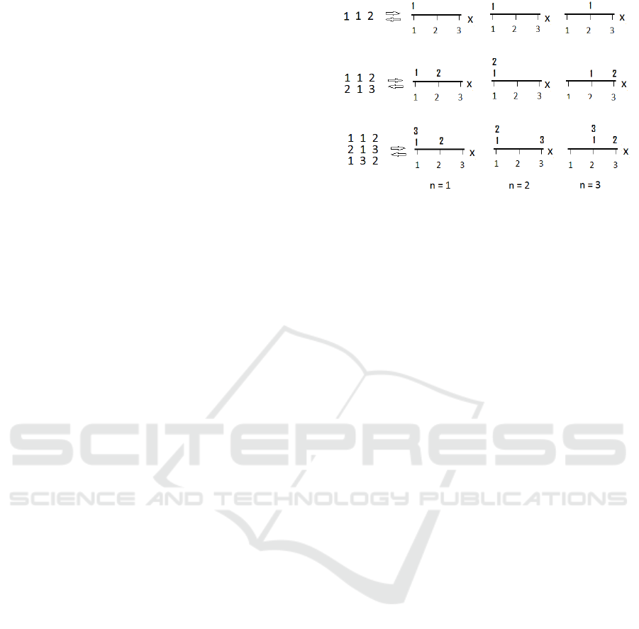
For an example, refer to Figure 2.
Figure 2: Three iterations involving growing columns that
graphically represent inverse patterns.
For this example, the indexes 1, 2, 3 of the patterns
123
(1,1,2) , (2,1,3) , (1,3,2)
are stored in
respective columns. For instance,
3, 2
{} {3}
xn
k
==
=
1, 1
{} {3,1}
xn
k
==
=
,
1, 3
{}
xn
k
==
=Æ
.
A notion of inverse patterns was introduced in
(Mikhailov, A. et al., 2017) and further discussed in
(Mikhailov, A. and Karavay, M., 2019). This notion
is related to inverse files technology used in Google
search engine (Brin, S. and Page, L., 1998) and in
the bag-of-words approach (Sivic, J. and Zisserman,
A., 2009). Whereas the latter approach recasts visual
object retrieval as text retrieval, the indextron
evaluates class probabilities of visual objects and
other objects such as sets, etc. by analyzing inverse
patterns of numeric features. For example, the
features a, b, c from indexed sets
12
{, }, {, }ab bc
are associated with the inverse sets
{1} , {1, 2} , {2}
abc
, which indicate that the feature
a belongs only to the set 1, the feature b belongs to
both the set 1 and the set 2, whereas the feature c
belongs only to the set 2.
For patterns, inverse pattern of a feature
x
is a set
{}
x
k
of classes
k
associated with this feature. So,
for two classes А,
А, А and Т, Т, the feature
“horizontal line” takes part in both A- and T-classes
whereas the feature “vertical line” takes part only in
class T:
0
{,}
A
T
o
,
90
{}T
o
.
The value of
R
in the transform (2) controls a
generalization capability of the classifier. Although
the total number
K of classes grows as new patterns
arrive, the rate of growth is inverse proportional to
generalization radius
R
.
ICPRAM 2021 - 10th International Conference on Pattern Recognition Applications and Methods
146
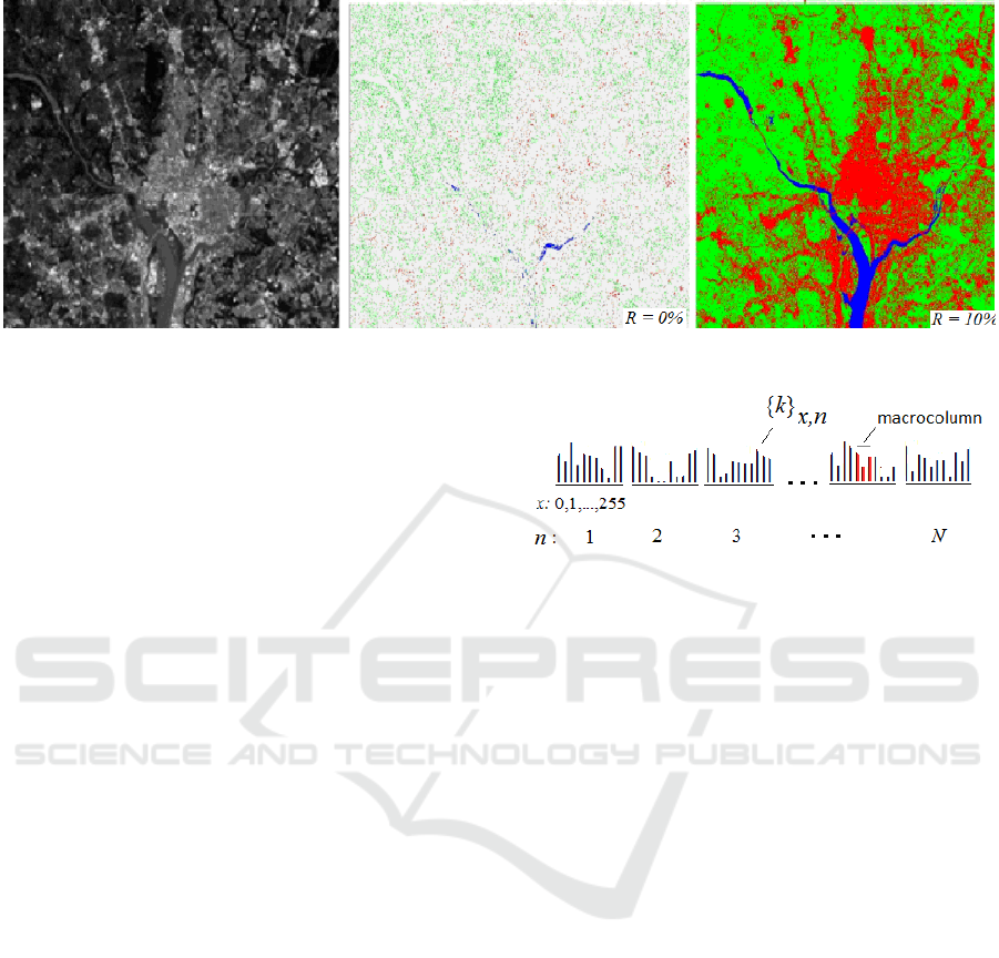
Figure 3: Image segmentation.
4.3 Generalization Radius
In accordance with the definition (1), any feature
change
112 2
, ,...,
NN
xx x+D +D +D
, such that
a variation
|| , 1,2,..,
n
Rn ND£ =
, does not
affect a pattern’s class. An influence of the radius
R
is shown on Figure 3. For this application, the pixels
of the left-hand side image are to be classified into 3
classes (water, vegetation, urban development).
Each pixel of the left-hand-side is represented by a
4-dimensional vector comprising components in the
256-level range in red, green, blue and infrared
spectra (only one component is shown). For original
images, refer to Gonzalez, R. and Woods, R. (2008).
The image at the center shows the segmentation
result at
0R =
, where most pixels remain
unclassified. The right-hand side image shows a
high quality image segmentation at
10%R = of
256-brightness range.
4.4 Indextron Architecture
The main parameters of the indextron are: the
pattern dimensionality
N
, the feature range
X
and
the maximum number
K of classes that can be
created by the classifier. In other words, the
indextron comprises
N groups of addresses, where
each group
n
contains
X
addresses ranging from
0 to 1
X
- . Typically, the normalized integer
feature range
X
is
[0,1, 2,..., 255]
. Each address
(, )
x
n is a gateway to the inverse pattern
,
{}
x
n
k
referred to as column (Figure 4).
Figure 4: N groups of indextron columns presenting a
cardinality distribution of inverse patterns.
Each column holds class indexes
k
, so that a column
height is equal to the cardinality of the
corresponding inverse pattern. A macro-column is
defined by the generalization radius
R
and contains
the neighboring columns with addresses from the
interval
[-, ]
x
Rx R+ .
In Figure 4, inverse patterns are shown as
N
groups of columns, each group containing
X
columns. The average column height
h
does not
account for 0-height columns. With classification
computational complexity of
()OhN , a flat
cardinality distribution of the inverse patterns is
preferable to a delta-like distribution.
A parallel processing of
N
column groups can
be implemented in a FPGA-chip, which leads to a
practically instantaneous learning. A memory that
needs to be allocated to column groups can be
arrange in three ways, that is, (a) static columns, (b)
dynamically allocated columns, (c) iterated one-
dimensional maps (Dmitriev A. et al., 1991;
Andreev et al., 1992). These methods would require
K
XN , 2
K
N and
K
N memory cells, respectively.
The method (c) makes possible an FPGA-
implementation of the
(, , )
K
XN
= (512, 256,
1024) indextron with a 1,44 MB chip (Figure 5).
Indextron
147
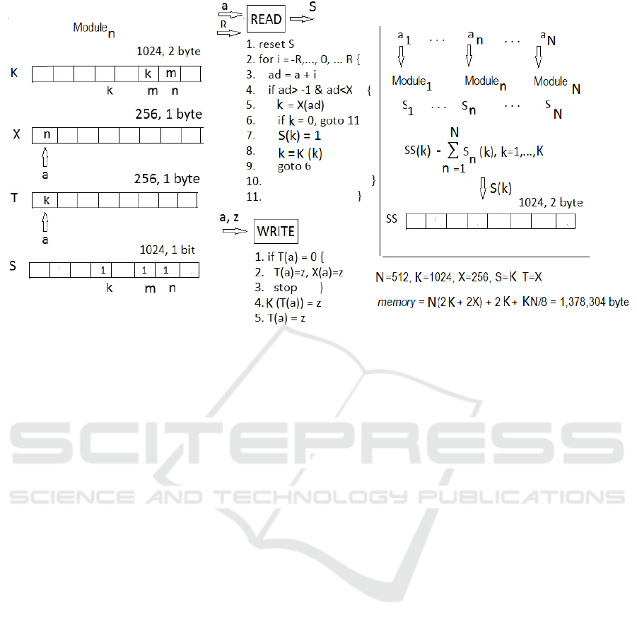
Figure 5: Indextron conceptual diagram.
In this case the total memory can be divided into
N groups of four arrays (N, X, T, S) plus the
common array SS. The total memory
M
amounts to
(2 /8) 2 (byte) MKNXTN N=++++
A normalized discrete feature range of X = 256 has
been found to be sufficient for most pattern
recognition applications meaning that
both float
point features and integer features can be converted
to 256 discrete levels without sacrificing an overall
accuracy.
In such implementation scheme
N identical
modules work in parallel. The component
n
a
of the
feature vector
1
,..., ,...,
nN
aaa
serves as the address
to the 256-byte array
X
of the
n
-th module.
On inference, the READ-code is executed (see
Figure. 5). The module’s output is a 1024-bit
word
n
S
. Next,
N
outputs are to be summed up
producing the 1024-element array
SS
, whose
elements are represented by 2-byte words
1
( ) ( ), 1, 2,...,
N
n
SS k S n k K
=
==
å
This array contains a conditional class distribution.
On learning, the WRITE-code is executed.
Again, the component
n
a
of the feature vector
1
,..., ,...,
nN
aaa
serves as the address to the 256-byte
array
X
of the
n
-th module, where the class index
z will be stored.
ACKNOWLEDGEMENTS
We thank Prof. Tanifuji, Riken Brain Science
Institute, for the permission to reproduce the image
of the IT-cortical region of a monkey (Figure 1, IT).
REFERENCES
Theodoridis S. & Koutroumbas K. (2006). Pattern
Recognition, Academic Press (3
rd
edition).
Tsunoda K., Yamane Y., Nishizaki M., Tanifuji M.,
(2001). Complex objects are represented in macaque
inferotemporal cortex by the combination of feature
columns. In Nat. Neurosci. 4 (8).pp.832-838.
doi:10.1038/90547. PMID 11477430
Les Chats. (2010). Retrieved from http://chatset
chiens3005.kazeo.com/les-chats-a122215626
Krizhevsky A., Nair V., Hinton G., (2009). CIFAR-10.
Retrieved from https://www.cs.toronto.edu/~kriz/
cifar.html
Chang D,. Canny J,. (2014). Optimizing Random Forests
on GPU. Tech. Report No. UCB/EECS-2014-2095.
Retrieved from http://www.eecs.berckeley.edu/Pubs/Tech
Rprts/2014/Eecs-2014-205.html
ICPRAM 2021 - 10th International Conference on Pattern Recognition Applications and Methods
148

Keras (2019). Retrieved from https://keras.io
Imagenet (2016). Retrieved from http://image-net.org
Mikhailov A., Karavay M., Farkhadov M. ( 2017). Inverse
Sets in Big Data Processing. In Proceedings of the
11th IEEE International Conference on Application of
Information and Communication Technologies
(AICT2017, Moscow). М.: IEEE, Vol. 1
https://www.researchgate.net/publication/321309177_
Inverse_Sets_in_Big_Data_Processing
Mikhailov A.and Karavay M. (2019). Pattern Recognition
by Pattern Inversion. In Proceedings of the 2nd
International conference on Image, Video
Processing and Artificial Intelligence, Shanghai, China.
SPIE Digital Library V.11321.
Brin S.and Page L. (1998). The Anatomy of a large-scale
hypotextual web search engine. In Computer Networks
and ISDN Systems Volume 30, Issues 1–7. Stanford
University, Stanford, CA, 94305, USA. Retrieved
from https://doi.org/10.1016/S0169-7552(98)00110-X
Sivic J., Zisserman A. (2009). Efficient visual search of
videos cast as text retrieval. In IEEE Transactions on
Pattern Analysis and Machine Intelligence Volume:
31, Issue: 4. doi: 10.1109/TPAMI.2008.111
Gonzales R. & Woods R., (2008). Digital Image
Processing. Pearson Prentice Hall (3rd edition).
http://www.imageprocessingplace.com/root_files_V3/i
mage_databases.htm
Dmitriev A., Panas A., Starkov S. (1991). Storing and
recognizing information based on stable cycles of one-
dimentional maps. In Phys. Lett. .
Andreev Y., Dmitriev A., Chua L, Wu C. (1992).
Associative and random access memory using one-
dimensional maps. In International Journal of
Bifurcation and Chaos vol.2, No 3. World Scientific
Publishing Company.
Indextron
149
