Solving Maximal Stable Set Problem via Deep Reinforcement Learning
Taiyi Wang
1
and Jiahao Shi
2
1
Department of Computer Science, Johns Hopkins University, Baltimore, MD, U.S.A.
2
Department of Applied Mathematics and Statistics, Johns Hopkins University, Baltimore, MD, U.S.A.
Keywords:
NP-hard, Maximal Stable Set, Deep Reinforcement Learning.
Abstract:
This paper provides an innovative method to approximate the optimal solution to the maximal stable set prob-
lem, a typical NP-hard combinatorial optimization problem. Different from traditional greedy or heuristic
algorithms, we combine graph embedding and DQN-based reinforcement learning to make this NP-hard opti-
mization problem trainable so that the optimal solution over new graphs can be approximated. This appears to
be a new approach in solving maximal stable set problem. The learned policy is to choose a sequence of nodes
incrementally to construct the stable set, with action determined by the outputs of graph embedding network
over current partial solution. Our numerical experiments suggest that the proposed algorithm is promising in
tackling the maximum stable independent set problem.
1 INTRODUCTION
In computational complexity theory, NP-hardness
(non-deterministic polynomial-time hardness) is the
defining property of a class of problems that are in-
formally “at least as hard as the hardest problems in
NP”. As it is suspected that P 6= NP, it is unlikely that
there exists an algorithm solving NP-hard problems
in polynomial time (Bovet et al., 1994).
Reinforcement learning (RL) is an area of ma-
chine learning concerned with how software agents
ought to take actions in an environment in order to
maximize the notion of cumulative reward. This
learning process differs from supervised learning in
not needing labelled input/output pairs be presented,
and in not needing sub-optimal actions to be explicitly
corrected (Kaelbling et al., 1996). Instead the focus
is on finding a balance between exploration (of un-
charted territory) and exploitation (of current knowl-
edge), and the application of RL is one of the hottest
topics in recent years. Deep Q-network (DQN) (Mnih
et al., 2015), an approach that trains deep neural net-
works to develop a novel artificial agent, can learn
successful policies directly from high-dimensional
sensory inputs using end-to-end reinforcement learn-
ing.
In graph theory, stable set (independent set) is a set
of vertices in a graph, no two of which are adjacent.
That is, it is a set S of vertices such that for every two
vertices in S, there is no edge connecting the two. The
size of an independent set is the number of vertices it
contains.
Maximal stable set is an independent set that is
not a subset of any other independent set. In other
words, there is no vertex outside the independent set
that may join it because it is maximal with respect
to the independent set property. Figure 1 shows six
different maximal independent sets (stable sets) and
two of them are maximum, marked as the red vertices.
Figure 1: MSS problem examples, red vertices form the
maximal stable sets.
The problem of finding such a set is called the maxi-
mum stable set (MSS) problem. This problem is com-
plementary to find the maximum clique of the graph.
A clique of an undirected graph is a subset of the ver-
tices, such that every two distinct vertices are adja-
cent. A set of a graph is independent if and only if it
is a clique in its complement. As a basic graph op-
Wang, T. and Shi, J.
Solving Maximal Stable Set Problem via Deep Reinforcement Learning.
DOI: 10.5220/0010179904830489
In Proceedings of the 13th International Conference on Agents and Artificial Intelligence (ICAART 2021) - Volume 2, pages 483-489
ISBN: 978-989-758-484-8
Copyright
c
 2021 by SCITEPRESS – Science and Technology Publications, Lda. All rights reserved
483

timization problem, MSS has many real-life applica-
tions such as wireless networks and DNA sequencing
(Joseph et al., 1992; Butenko and Pardalos, 2003).
There are several existing approaches that attempt
to solve the MSS problem, including sequential al-
gorithm, random-priority parallel algorithm, random-
permutation parallel algorithm (Blelloch et al., 2012),
maximum satisfiability solvers (Li and Quan, 2010),
etc. However, the MSS problem is an NP-hard opti-
mization problem and the above-mentioned methods
are all greedy or heuristic algorithms in nature. As
such, it is unlikely that there exists an extremely ef-
ficient algorithm for finding a maximum independent
set of a graph.
Recently, DQN-based reinforcement learning is
used in approximating optimal solutions for combi-
natorial optimization problems (Khalil et al., 2017;
Bello et al., 2016). This idea is motivated by the fact
that real-world optimization problem maintains simi-
lar combinatorial structure but only differs in the data.
This inherent similarity among problem instances ap-
pears to also exist in the MSS problem. It is common
to find that two different MSS problem have similar
combinatorial structures, especially when they arise
in the same domain. This motivates us to train the
MSS problem over a number of randomly generated
graphs that may have a resemblance to unseen real-
world graphs or networks.
In this paper, we consider using graph embedding
and reinforcement learning to approximate the opti-
mal solution to MSS problems. Notice that although
the framework of combining graph embedding and
reinforcement learning has already been used to ap-
proximate the minimum vertex cover set, a comple-
ment of the MSS, of a graph. It is not trivial to ap-
proximate the optimal solution to the MSS problem
since the complement of an estimated minimum ver-
tex cover set is not always an MSS of a graph. Hence,
establishing a new framework for the MSS problem is
necessary.
2 DEEP REINFORCEMENT
LEARNING FRAMEWORKS
2.1 Problem Description
Given a graph G = (V, E), find a subset of nodes S ⊆
G such that no two edges in S are adjacent, and |S| is
maximized.
Let S = (v
1
,··· , v
|S|
) denote a partial solution,
where v
i
∈ V represents the nodes of S, and
¯
S = V \S
the set of candidate nodes to be added. We also use
S to describe the current state of G. Let x represent
a tag of G with the current partial solution S, with
each dimension x
v
= 1 if the node v ∈ S and 0 oth-
erwise. We consider using a maintenance procedure
h(S) which maps an ordered list S to a combinatorial
structure satisfying the specific constraints of a prob-
lem. This maintenance procedure is a standard pro-
cedure in previous research (Khalil et al., 2017). In
our problem setting, the helper functionh(·) is unnec-
essary, because our target is to find a stable set with
the largest size, the quality of a partial solution S can
be simply defined as |S|.
In our framework, we rely on a greedy algorithm,
a popular approach in designing approximation al-
gorithms, that constructs a solution by sequentially
adding nodes to a partial solution. The policy of
choosing which node to be added for each iteration
is determined by some evaluation function Q(h(S),v)
that measures the quality of adding a node to the cur-
rent partial solution. Then, the algorithm will extend
the partial solution S as:
S
:
= (S,v
∗
), where v
∗
= arg max
v∈
¯
S
Q(h(S),v).
2.2 Representation
Graph Embedding. Because we are optimizing
over a graph G = (V,E), we expect that the evalu-
ation function Q should take into account the infor-
mation of G, its current state S and the node v to be
added. The difficulty of expressing Q(h(S), v) moti-
vates us to design a powerful deep learning approxi-
mator
ˆ
Q(h(S),v; Θ) with parameters Θ to estimate the
Q function learned from a collection of problem in-
stances. The problem instances are obtained by gen-
erating a set of graphs {G
i
}
m
i=1
from a distribution D.
In particular, we choose to use structure2Vec as the
graph embedding network due to its effectiveness in
representing structured data (Dai et al., 2016).
We follow (Khalil et al., 2017) to implement graph
embedding. Let µ
v
, a p-dimensional vector, repre-
sent the embedding of node v. Given a graph frame-
work, a network structure is recursively defined by the
stucture2Vec. Specifically, it would begin with initial
embedding µ
v
0
at each node, and then for all v in V
updating the embedding synchronously at each iter-
ation, so the next µ
v
is calculated by a generic non-
linear function with parameters related to the graph.
Then node-specific tags x
v
are aggregated recursively
according to G’s graph topology. After a few steps
of recursion, the network will produce a new embed-
ding µ
v
for each node, taking into account both graph
characteristics and long-range interactions. This pro-
ICAART 2021 - 13th International Conference on Agents and Artificial Intelligence
484

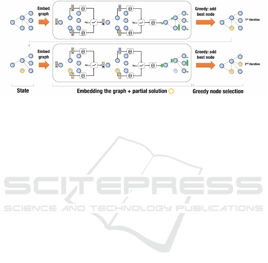
Figure 2: Illustration of the proposed framework as applied to an instance of Maximal Stable Set. The middle part illustrates
two iterations of the graph embedding, which results in node scores (green bars).
cedure is formalized as
µ
v
t+1
← F(x
v
,{µ
u
t+1
}
u∈N(v)
,{w(v,u)}
u∈N(v)
;Θ),
where N(v) is the set of neighbors of node v in G,
and F is a generic nonlinear mapping such as a neu-
ral network or kernel function. An illustration of two
iterations of graph embedding can be found in Figure
2.
Parameterizing Q Function. Now, we come to the
parameterization procedure of
ˆ
Q(h(S),v; Θ) which fa-
cilitates applying deep neural networks. The function
to update a p-dimensional embedding µ
v
works as fol-
lows:
µ
v
t+1
← relu(θ
1
x
v
+ θ
2
∑
u∈N(v)
µ
u
t
+ θ
3
∑
u∈N(v)
relu(θ
4
w(v,u)),
where θ
1
∈ R
p
, θ
2
, θ
3
∈ R
p×p
and θ
4
∈ R
p
are four
parameters used in this model, w(v, u) represents the
edge weight of the graph where all the entries are 1 in
our problem and relu function (relu(z) = max(0, z))
is a type of activation function which is applied to in-
crease nonlinear transformations.
After T iterations of the embedding of each node,
we obtain the embedding µ
v
T
for node v. We also ob-
tain the pooled embedding
∑
u∈V
µ
u
T
over the whole
graph. µ
v
T
and
∑
u∈V
µ
u
T
corresponds to the embed-
ding maps of v and h(S).
ˆ
Q(h(S),v; Θ) can then be
parameterized as
ˆ
Q(h(S),v; Θ) = θ
5
T
relu([θ
6
∑
u∈V
µ
u
T
,θ
7
µ
v
T
]),
where θ
5
∈ R
2p
, θ
6
, θ
7
∈ R
p×p
. And within the relu
function, we concatenate θ
6
∑
u∈V
µ
u
T
and θ
7
µ
v
T
.
Since we assume that there is no ground truth la-
bel for every input graph G in our approach, these 7
parameters have to be trained by using reinforcement
learning method.
2.3 Deep Q-learning
2.3.1 Reinforcement Learning Formulation
We define the state, action, and reward in the rein-
forcement learning framework as follows:
1. State: a state S is a sequence of actions (nodes) on
a graph G that forms a stable set. And the terminal
state S
∗
is achieved when we cannot add any more
node to S
∗
.
2. Transition: a transition from S to S
0
is determinis-
tic here, and corresponds to tagging the node that
was selected as the last action by setting x
v
= 1
for v being last action. In addition, the update of
candidate pool removes all node v
0
that is adjacent
to v.
3. Candidate Pool: the candidate pool, denoted as
C, is a collection of node, such that for ∀v ∈ C,
@ v
0
∈ S with e = vv
0
∈ E (e denotes the connection
between node v and v
0
) and v /∈ S.
4. Action: an action v is a node of G that is in can-
didate pool C. And we will use p-dimensional
embedding µ
v
to represent action v, and this rep-
resentation is applicable across graphs.
5. Reward: for maximum stable set problem, a re-
ward of action v is just the increment of the size
of state.
6. Policy: based on
ˆ
Q, we use a deterministic greedy
policy
π(v|S) = argmax
v
0
∈
¯
S
ˆ
Q(h(S),v
0
).
Solving Maximal Stable Set Problem via Deep Reinforcement Learning
485

7. Episode: an episode is a complete sequence of ad-
ditions starting from empty solution, and until ter-
mination for a graph G.
8. Step: a step within each episode is a single node
addition.
2.3.2 Training
We are trying to build a reinforcement learning frame-
work to approximate our maximum stable set prob-
lem. we have two different networks to address our
problem.
The first network is a class called S2V, which is
used to implement the graph embedding function us-
ing structure2Vec. The second network takes the em-
bedding for each node as input and return the value of
ˆ
Q(h(S),v; Θ).
Our graph embedding parameters in
ˆ
Q(h(S),v; Θ)
are learned via a standard 1-step Q-learning update.
The update of function parameters at each step of an
episode is to perform a gradient step to minimize the
squared loss:
(y −
ˆ
Q(h(S
t
),v
t
,Θ))
2
, (1)
where y = γ max
v
0
ˆ
Q(h(S
t+1
),v
0
;Θ) + r(S
t
,v
t
) for a
non-terminal state S
t
. And instead of updating Q-
function sample-by-sample as in equation (1), we
update the function with a batch of samples from
dataset E, rather than the single sample being cur-
rently experienced. The dataset E is populated dur-
ing previous episodes, such that at step t + 1, the tuple
(S
t
,v
t
,r(S
t
,v
t
),S
t+1
) is added to E, and the stochastic
gradient descent updates are performed on a random
sample of tuples drawn from E. And the whole greedy
Q-learning procedures are shown in Algorithm 1 be-
low.
2.4 Code Implementation
We built our code based on Pytorch Framework and
ran our python program on a CUDA capable GPU.
Our code sharing on Google Colaboratory provides
users with an easy entry into free GPU-accelerated
computing, as we copied all the network structures
(refer to Q.py) and the tensor variables (refer to
Agent.py) to the GPU specified device at the begin-
ning, and the subsequent operations were performed
on the GPU as well
1
. We also offer our open source
code in the Github
2
. Notice that we also provide
1
Link to the Google Colab repo: https://drive.google.
com/drive/folders/1EAxBpWfuDVBISbuxDoOAs3
nB5qFpOIV?usp=sharing
2
Please refer to the link: https://github.com/
Kevinwty0107/DQN-MSS
Algorithm 1: Q-learning for the Greedy Algorithm.
1: Initialize experience replay memory M to capac-
ity N
2: for episode e = 1 to L do
3: Draw graph G from distribution D
4: Initialize the state to empty S
1
=
/
0
5: for step t = 1 to T do
6: v
t
=
(
random node v ∈ C
t
(w.p.ε)
argmax
v∈C
t
ˆ
Q(h(S
t
),v; Θ) (O.W)
7: Add v
t
to partial solution S
t+1
:= (S
t
,v
t
)
8: Update C
t+1
by removing neighbor of v
t
from C
t
9: Add tuple (S
t+1
,v
t
,r(S
t
,v
t
),S
t
) to M
10: Sample random batch B
i.i.d
∼ M
11: Update Θ by SGD over (1) for B
12: end for
13: end for
14: return Θ
with a Greedy algorithm in the Google Colab and the
Github.
When training with the mini-batch method, the
acceleration performance of GPU has obviously im-
proved the speed of running neural networks. This
is why when the number of nodes increases and the
high-performance GPUs are introduced, either mul-
tiple GPUs in parallel or a single GPU, the running
time of our neural network will be significantly re-
duced. The improvements brought by GPU can be
shown by numerical experiments: When nodes = 20,
We used single Tesla P4 GPU and i7-7700K CPU
to run our code with 10w episodes simultaneously.
The GPU took about 45 minutes while the CPU took
nearly 80 minutes in the training phase, i.e., GPU im-
proved the speed by 78%, indicating that running on
GPU is significantly faster than CPU. When nodes =
40, GPU improved the speed by 90%. Previous al-
gorithms proposed in the MSS problem are all imple-
mented on CPUs, though they use methods like ex-
act branch-and-bound algorithm and are able to reach
high approximating ratio, when scaling to hundreds of
nodes, the speed of running with these classic meth-
ods would be extremely slow and Deep-RL will out-
perform them.
ICAART 2021 - 13th International Conference on Agents and Artificial Intelligence
486

3 EXPERIMENTAL &
COMPUTATIONAL RESULTS
3.1 Dataset Used and Input/Output
Streams
To evaluate the proposed algorithm against other ap-
proximation/heuristic algorithms, we generate graph
instances for our MSS problem using Erdos-Renyi
(ER) (Erd
˝
os and R
´
enyi, 1960) and Barabasi-Albert
(BA) (Albert and Barab
´
asi, 2002) graph-generation
models which have been used to model many real-
world networks.
Our input Graph file could be recorded as G(V,E),
and stored in COO form. When the graphs are used
for test on Cliquer programs, we convert them into
DIMACS format, which is a common format for de-
scribing graphs on which Cliquer Tools can be easily
applied.
Our output files are stored in .txt files in the
score result folder, containing all the output results
obtained from our Deep-RL model, and the Greedy
algorithm with episode index, number of nodes, the
score (size of the maximum stable set found) and the
set of nodes at each line.
3.2 Test & Compare Our Results with
Cliquer and Greedy Algorithm
To test and compare our results with other algorithms,
an open source tool Cliquer
3
is introduced, which
is mainly built based on the branch-and-bound algo-
rithm.
At the same time, the Greedy algorithm is intro-
duced in the comparison as well, where the nodes of
a graph are first ordered by their degrees (that is, the
number of neighbors), and then they are processed in
order (starting with the lowest degree), the next node
to the target stable set S will be added if it has no
neighbors in S.
3.3 Result Tables and Plots
To show the evaluation and comparison results for dif-
ferent algorithms, we present several tables and plots .
Table 1 and Table 2
4
show the comparison results be-
3
Cliquer tool, developed by Patric
¨
Osterg
˚
ard, please re-
fer to https://users.aalto.fi/ pat/cliquer.html for more details.
The execution file Basic in our project is used for find-
ing Maximum Cliques of any given graphs formed by non-
isolated points.
4
Lines with red numbers mean the same size given by
both methods
tween our Deep-RL model and the Cliquer and the
Greedy algorithm over a collection of graphs, and
they are produced under conditions of “node num =
15, training episode = 10000” and “node num = 30,
training episode = 50000”, respectively.
It can be concluded that, when the number of
graph nodes equals 15, all three algorithms give out
the same stable set, and when the number of graph
nodes increases and equals 30, our trained Deep-RL
model may fall into the local optimum and report a
solution that is not a maximum stable set. This can
be understood as, given the same number of training
episode, the smaller the graph is, the easier it will be
trained to be more accurate. On the other hand, when
the number of training episode increases, our model
will perform better. For the Deep-RL method, it is
worth mentioning that although we need additional
time to train the network, we will save a lot of time
and space compared to the heuristic and the greedy
algorithms when we look for the MSS of the graph
in the pool using our trained networks. Regardless
of additional time cost, using a pre-trained Deep-RL
model appears to outperform other two algorithms in
computing time, especially when the number of nodes
gets larger.
Table 1: Algorithm comparison of MSS size over six graph
instances (node num = 15, training episode=10000).
Nodes Cliquer Size Greedy Size RL Size
15 6 6 6
15 7 7 7
15 8 8 8
15 5 5 5
15 7 7 7
15 6 6 6
Table 2: Algorithm comparison of MSS size over four graph
instances (node num = 30, training episode=50000).
Nodes Cliquer Size Greedy Size RL Size
30 12 12 12
30 12 12 11
30 13 13 13
30 9 9 8
To evaluate our results in a larger number of graph
instances, figure 3 and figure 4 below show the qual-
ity comparison among different algorithms. Figure 5
presents the log loss curve during training process, in
which you can see an obvious decreasing (to conver-
gence) curve and the stability of the training process.
Solving Maximal Stable Set Problem via Deep Reinforcement Learning
487

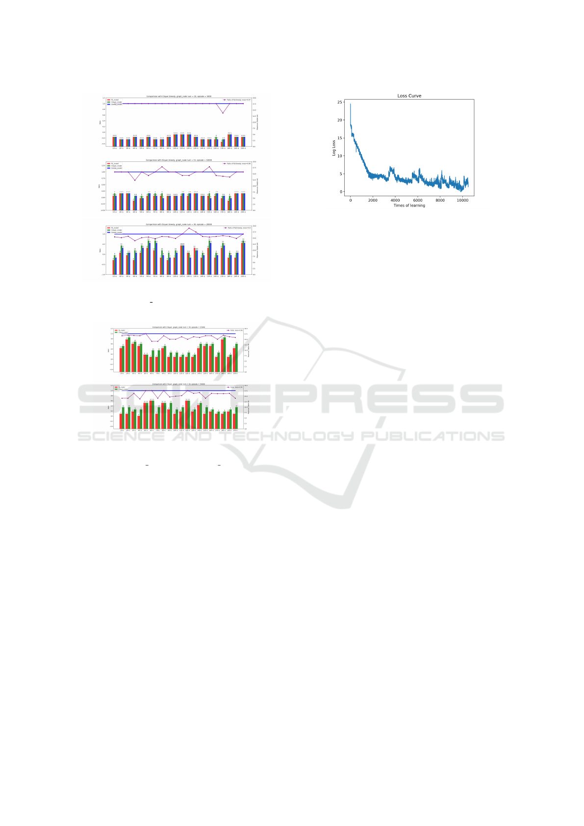
Figure 3: Algorithm comparison of MSS size over 20 graph
instances, where node num =10 (top), 15 (middle), 30 (bot-
tom).
Figure 4: Algorithm comparison between the Deep-RL
and the Cliquer algorithm of MSS size over 20 graph in-
stances, where node num = 30, training episode = 15000
(top), 50000 (bottom).
4 CONCLUSIONS AND FURTHER
DISCUSSIONS
In our paper, deep reinforcement learning, an end-
to-end machine learning enhanced method which can
applied in tackling NP-hard combinatorial optimiza-
tion problems on graphs, is introduced. Central to our
approach is the combination of deep graph embed-
ding and reinforcement learning method. Through
extensive experimental evaluations, we demonstrate
the effectiveness of our proposed framework in learn-
ing greedy heuristics. The performance of the learned
heuristics is consistent across multiple different graph
types, and graph sizes, suggesting that S2V-DQN
framework is a promising new tool for MSS prob-
lems. For the future work, there are some discussions
as follows.
First, although we have designed a complete
Figure 5: Log Loss Curve during training.
implementation pipeline of the deep reinforcement
learning algorithm and our numerical results have
demonstrated that it seems to be a very effective
tool to approximate the optimal solution to the MSS
problem, we still need to make more comparisons
to illustrate the superiority of this method over the
existing algorithms. When the graph size is rela-
tively small, the traditional methods like Cliquer and
Greedy may perform better due to the additional train-
ing cost brought by Deep-RL. However, the strength
of Deep-RL is that we can train the large graphs on
high-performance GPUs in scale, which means when
the size of graphs gets larger, the time needed to find
solutions of methods like Cliquer or Greedy becomes
longer while the speed by using Deep-RL may outper-
form other methods. Limited to the page restriction
of the article and the computational resources, we are
not able to present the experiments’ results over large-
scale data. Moreover, given our complete testing en-
vironment and the trained networks, we can evaluate
our proposed algorithm from many other aspects in
the future, such as running time and the performance
consistency under arbitrary graph size.
Second, our network structure is designed based
on the intuition of previous experiences in approx-
imating other combinatorial optimization problems.
We mainly apply linear layers in our deep neural
networks in this work. For future improvements,
we may explore a better network structure or graph-
embedding framework to achieve an overall higher
performance.
Third, the idea proposed in this paper can not only
applied to the MSS problem but also used in many
other combinatorial optimization problems. Since
there is a strong coupling between graph-based opti-
mization and real-world problems, we can find some
scenarios where our algorithm is really useful, such
as transforming the facility location problem into a
problem of finding a feasible subset. When dealing
with real-world applications, the key is that we need
to formalize our problem space and improve models’
performances when applying over large data sets.
ICAART 2021 - 13th International Conference on Agents and Artificial Intelligence
488

REFERENCES
Albert, R. and Barab
´
asi, A.-L. (2002). Statistical mechan-
ics of complex networks. Reviews of modern physics,
74(1):47.
Bello, I., Pham, H., Le, Q. V., Norouzi, M., and Bengio, S.
(2016). Neural combinatorial optimization with rein-
forcement learning. arXiv preprint arXiv:1611.09940.
Blelloch, G. E., Fineman, J. T., and Shun, J. (2012). Greedy
sequential maximal independent set and matching are
parallel on average. In Proceedings of the twenty-
fourth annual ACM symposium on Parallelism in al-
gorithms and architectures, pages 308–317.
Bovet, D. P., Crescenzi, P., and Bovet, D. (1994). Intro-
duction to the Theory of Complexity. Prentice Hall
London.
Butenko, S. and Pardalos, P. M. (2003). Maximum indepen-
dent set and related problems, with applications. PhD
thesis, University of Florida.
Dai, H., Dai, B., and Song, L. (2016). Discriminative
embeddings of latent variable models for structured
data. In International conference on machine learn-
ing, pages 2702–2711.
Erd
˝
os, P. and R
´
enyi, A. (1960). On the evolution of random
graphs. Publ. Math. Inst. Hung. Acad. Sci, 5(1):17–
60.
Joseph, D., Meidanis, J., and Tiwari, P. (1992). Determin-
ing dna sequence similarity using maximum indepen-
dent set algorithms for interval graphs. In Scandina-
vian Workshop on Algorithm Theory, pages 326–337.
Springer.
Kaelbling, L. P., Littman, M. L., and Moore, A. W. (1996).
Reinforcement learning: A survey. Journal of artifi-
cial intelligence research, 4:237–285.
Khalil, E., Dai, H., Zhang, Y., Dilkina, B., and Song, L.
(2017). Learning combinatorial optimization algo-
rithms over graphs. In Advances in Neural Informa-
tion Processing Systems, pages 6348–6358.
Li, C. M. and Quan, Z. (2010). An efficient branch-and-
bound algorithm based on maxsat for the maximum
clique problem. In AAAI, volume 10, pages 128–133.
Mnih, V., Kavukcuoglu, K., Silver, D., Rusu, A. A., Ve-
ness, J., Bellemare, M. G., Graves, A., Riedmiller, M.,
Fidjeland, A. K., Ostrovski, G., et al. (2015). Human-
level control through deep reinforcement learning. na-
ture, 518(7540):529–533.
Solving Maximal Stable Set Problem via Deep Reinforcement Learning
489