Latent Space Conditioning on Generative Adversarial Networks

Ricard Durall

1,2,3

, Kalun Ho

1,3,4

, Franz-Josef Pfreundt

and Janis Keuper

1,5

Fraunhofer ITWM, Germany

IWR, University of Heidelberg, Germany

Fraunhofer Center Machine Learning, Germany

Data and Web Science Group, University of Mannheim, Germany

Institute for Machine Learning and Analytics, Offenburg University, Germany

Keywords:

Generative Adversarial Network, Unsupervised Conditional Training, Representation Learning.

Abstract:

Generative adversarial networks are the state of the art approach towards learned synthetic image generation.

Although early successes were mostly unsupervised, bit by bit, this trend has been superseded by approaches

based on labelled data. These supervised methods allow a much ﬁner-grained control of the output image,

offering more ﬂexibility and stability. Nevertheless, the main drawback of such models is the necessity of

annotated data. In this work, we introduce an novel framework that beneﬁts from two popular learning tech-

niques, adversarial training and representation learning, and takes a step towards unsupervised conditional

GANs. In particular, our approach exploits the structure of a latent space (learned by the representation learn-

ing) and employs it to condition the generative model. In this way, we break the traditional dependency

between condition and label, substituting the latter by unsupervised features coming from the latent space.

Finally, we show that this new technique is able to produce samples on demand keeping the quality of its

supervised counterpart.

1 INTRODUCTION

Generative Adversarial Networks (GANs) (Goodfel-

low et al., 2014) are one of the most prominent un-

supervised generative models. Their framework in-

volves training a generator and discriminator model

in an adversarial game, such that the generator learns

to produce samples from the data distribution. Train-

ing GANs is challenging because they require to deal

with a minimax loss that needs to ﬁnd a Nash equilib-

rium of a non-convex function in a high-dimensional

parameter space. This scenario may lead to a lack

of control during the training phase, exhibiting non-

desired side effects such as instability, mode collapse,

among others. As a result, many techniques have been

proposed to improve the stability training of GANs

(Salimans et al., 2016; Gulrajani et al., 2017; Miyato

et al., 2018; Durall et al., 2019).

Conditioning has risen as one of the key technique

in this vein (Mirza and Osindero, 2014; Chen et al.,

2016; Isola et al., 2017; Choi et al., 2018), whereby

the whole model has granted access to labelled data.

In principle, providing supervised information to the

discriminator encourages it to behave more stable at

training since it is easier to learn a conditional model

for each class than for a joint distribution. However,

conditioning comes with a price, the necessity for an-

notated data. The scarcity of labelled data is a major

challenge in many deep learning applications which

usually suffer from high data acquisition costs.

Representation learning techniques enable models

to discover underlying semantics-rich features in data

and disentangle hidden factors of variation. These

powerful representations can be independent of the

downstream task, leaving the need of labels in the

background. In fact, there are fully unsupervised rep-

resentation learning methods (Misra et al., 2016; Gi-

daris et al., 2018; Rao et al., 2019; Milbich et al.,

2020) that automatically extract expressive feature

representations from data without any manually la-

belled annotation. Due to this intrinsic capability, rep-

resentation learning based on deep neural networks

have been becoming a widely used technique to em-

power other tasks (Caron et al., 2018; Oord et al.,

2018; Chen et al., 2020).

Motivated by the aforementioned challenges, our

goal is to show that it is possible to recover the bene-

ﬁts of conditioning by exploiting the advantages that

representation learning can offer (see Fig. 1). In par-

ticular, we introduce a model that is conditioned on

the latent space structure. As a result, our proposed

method can generate samples on demand, without ac-

Durall, R., Ho, K., Pfreundt, F. and Keuper, J.

Latent Space Conditioning on Generative Adversarial Networks.

DOI: 10.5220/0010178800240034

In Proceedings of the 16th International Joint Conference on Computer Vision, Imaging and Computer Graphics Theory and Applications (VISIGRAPP 2021) - Volume 4: VISAPP, pages

24-34

ISBN: 978-989-758-488-6

40 20 0 20 40

Dimension 1

Dimension 2

40 20 0 20 40

Dimension 1

Dimension 2

40 20 0 20 40

Dimension 1

Dimension 2

plane

car

bird

cat

deer

dog

frog

horse

ship

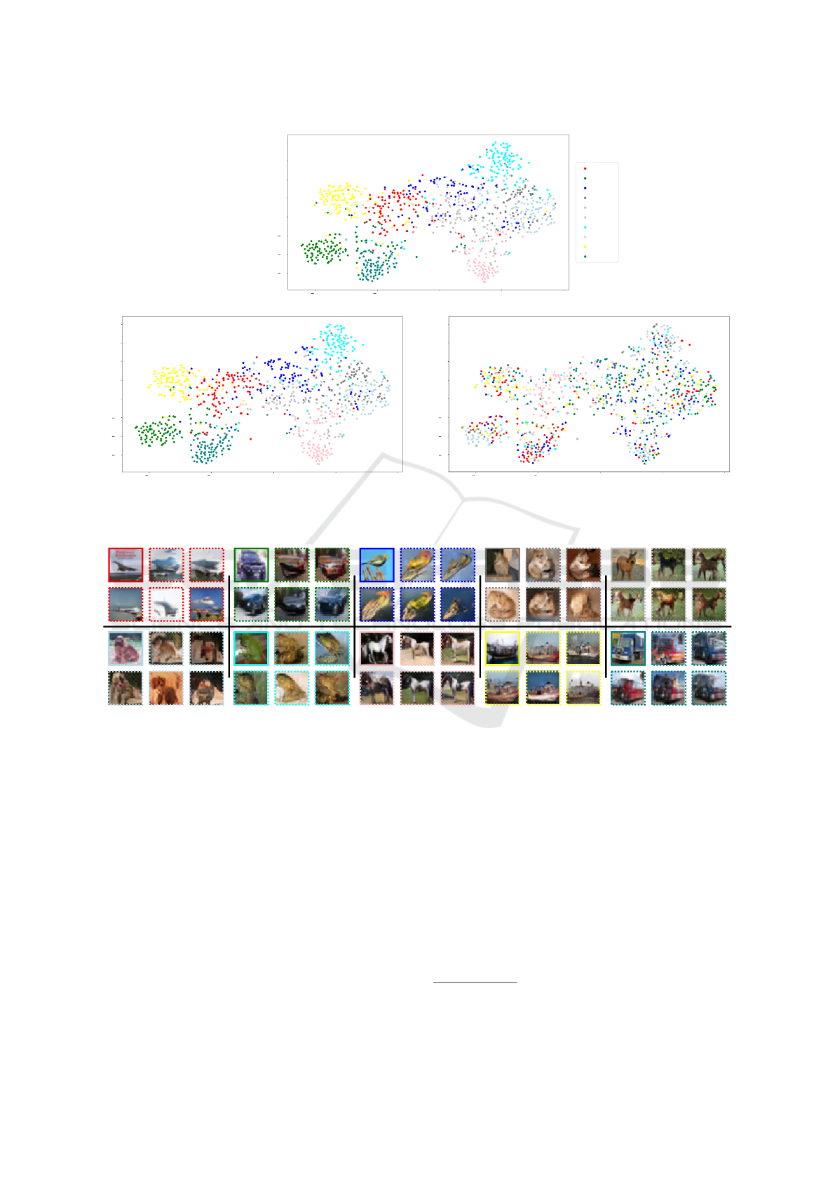
(a) t-SNE visualizations. Upper-Center: Original latent space. Bottom-Left: Latent space according to our approach. Bottom-

Right: Latent space according to standard approach

. Both bottom spaces represent the classes of the generated images given

a latent code. Therefore, they should be as similar as possible to the original latent space.

(b) Random sets of generated samples trained on CIFAR10. The solid frames contain real images and the dashed the generated.

Figure 1: Given a latent space, our approach exploits the structure using its features to condition the generative model. In this

way, our system eventually can produce samples on demand. The code color is consistent within the whole ﬁgure.

cess to labeled data at the GAN level. To ensure the

correct behaviour, a customized loss is added to the

model. Our contributions are as follows.

• We propose a novel generative adversarial net-

work conditioned on features from a latent space

representation.

• We introduce a simple yet effective new loss func-

tion which incorporates the structure of the latent

space.

• Our experimental results show a neat control on

the generated samples. We test the approach on

MNIST, CIFAR10 and CelebA datasets.

2 RELATED WORK

2.1 Conditional Generative Adversarial

Networks

Generative image modelling has recently advanced

dramatically. State-of-the-art methods are GAN-

based models (Brock et al., 2018; Karras et al., 2019;

Karras et al., 2020) which are capable of generat-

ing high-resolution, diverse samples from complex

Standard approach refers to replace the encoded labels

with latent code.

Latent Space Conditioning on Generative Adversarial Networks

datasets. However, GANs are extremely sensitive to

nearly every aspect of its set-up, from loss function

to model architecture. Due to optimization issues

and hyper-parameter sensitivity, GANs suffer from te-

dious instabilities during training.

Conditional GANs have witnessed outstanding

progress, rising as one of the key technique to im-

prove stability training and to remove mode collapse

phenomena. As a consequence, they have become

one of the most widely used approaches for gener-

ative modelling of complex datasets such as Ima-

geNet. CGAN (Mirza and Osindero, 2014) was the

ﬁrst work to introduce conditions on GANs, shortly

followed by a ﬂurry of works ever since. There have

been many different forms of conditional image gen-

eration, including class-based (Mirza and Osindero,

2014; Odena et al., 2017; Brock et al., 2018) , image-

based (Isola et al., 2017; Huang et al., 2018; Mao

et al., 2019) , mask- and bounding box-based (Hinz

et al., 2019; Park et al., 2019; Durall et al., 2020), as

well as text-based (Reed et al., 2016; Xu et al., 2018;

Hong et al., 2018). This intensive research has led

to impressive development of a huge variety of tech-

niques, paving the road towards the challenging task

of generating more complex scenes.

2.2 Unsupervised Representation

Learning

In recent years, many unsupervised representation

learning methods have been introduced (Misra et al.,

2016; Gidaris et al., 2018; Rao et al., 2019; Milbich

et al., 2020). The main idea of these methods is to ex-

plore easily accessible information, such as temporal

or spatial neighbourhood, to design a surrogate super-

visory signal to empower the feature learning. Al-

though many traditional approaches such as random

projection (Li et al., 2006), manifold learning (Hinton

and Roweis, 2003) and auto-encoder (Vincent et al.,

2010) have signiﬁcantly improved feature represen-

tations, many of them often suffer either from be-

ing computationally too costly to scale up to large or

high-dimensional datasets, or from failing to capture

complex class structures mostly due to its underlying

data assumption.

On the other hand, a number of recent unsuper-

vised representation learning approaches rely on new

self-supervised techniques. These approaches formu-

late the problem as an annotation free pretext task;

they have achieved remarkable results (Doersch et al.,

2015; Oord et al., 2018; Chen et al., 2020) and

even on GAN-based models as well (Chen et al.,

2019). Self-supervision generally involves learning

from tasks designed to resemble supervised learning

in some way, where labels can be created automati-

cally from the data itself without manual intervention.

3 METHOD

In this section we describe our approach in detail.

First, we present our representation learning set-up

together with its sampling algorithm. Then, we in-

troduce a new loss function capable of exploiting the

structural properties from the latent space. Finally, we

have a look at the adversarial framework for training

a model in an end-to-end fashion. Fig. 2 gives an

overview of the main pipeline and its components.

3.1 Representation Learning

The goal of representation learning or feature learn-

ing is to ﬁnd an appropriate representation of data in

order to perform a machine learning task.

Generating Latent Space. The latent space must

contain all the important information needed to rep-

resent reliably the original data points in a simpli-

ﬁed and compressed space. Similar to (Aspiras et al.,

2019), in our work we also try to exploit the latent

space. In particular, we rely on existing topologies

that can capture a high level of abstraction. Hence,

we mainly focus on integrating these data descriptors

and on evaluating their usability and impact. For this

reason, We count on several set-ups where we can

sample informative features of different qualities, i.e.

level of clustering in the latent spaces.

Our feature extractor block E is a convolutional-

based model for classiﬁcation tasks. Inspired by

(Caron et al., 2018), to extract the features we do not

use the classiﬁer output logits, but the feature maps

from an intermediate convolutional layer. We refer to

these hidden spaces as latent space.

Sampling from Latent Space. Assuming that the

feature extractor is able to produce a structured la-

tent space, e.g. semi-clustered features, we can start

sampling observations that will be fed to our GAN af-

terwards. The procedure to create sampling batches is

described in Algorithm 1.

3.2 Loss Function

Minimax Loss. A GAN architecture is comprised of

two parts, a discriminator D and a generator G. While

the discriminator trains directly on real and gener-

ated images, the generator trains via the discrimina-

tor model. They should therefore use loss functions

VISAPP 2021 - 16th International Conference on Computer Vision Theory and Applications

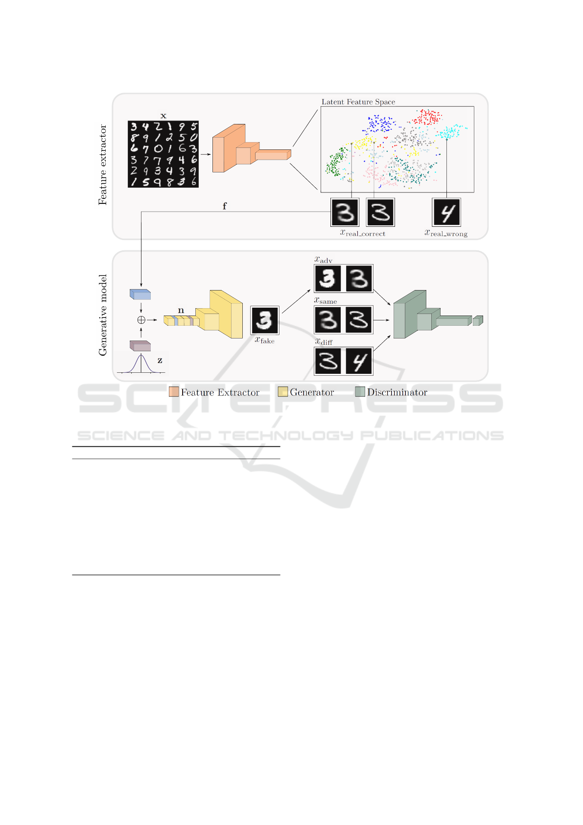
Figure 2: Overview of the processing pipeline of our approach. It contains two main blocks, a feature extraction model and a

generative model, more speciﬁcally a GAN. This structure allows the generator to incorporate a condition based on the latent

space, so that eventually the system can produce images on demand using the latent representation.

Algorithm 1: Creating batches for training the GAN.

1: Sample a batch of images x

2: Extract features from it f = E(x)

3: Compute distance between all features D = ||f||

4: for x

in x do

5: Select x

and sort the rest according to their dis-

tance d(x

)

6: Select nearest neighbour from x

, i.e. d

min

)

7: Select the farthest neighbour from x

, i.e.

max

)

8: end for

that reﬂect the distance between the distribution of

the data generated p

and the distribution of the real

data p

data

. Minimax loss is by default the candidate to

carry on with this task and it is deﬁned as

min

max

L (D, G) =E

x∼p

data

[log(D(x))]+

z∼p

[log(1 − D(G(z)))].

(1)

Triple Coupled Loss. In the vanilla minimax loss the

discriminator expects batches of individual images.

This means that there is a unique mapping between

input image and output, where each input is evaluated

and then classiﬁed as real or fake. Despite being a

functional loss term, if we hold to that closed formu-

lation, we cannot leverage alternatives such as condi-

tional features or combinatorial inputs i.e. input is not

any longer only a single image but a few of them.

We introduce a loss function coined triple cou-

pled loss that incorporates combinatorial inputs act-

ing as a semi-conditional mechanism. The approach

lies on the idea of exploiting similitudes and differ-

ences between images. In fact, similar approaches

have been already successfully implemented in other

works (Chongxuan et al., 2017; Sanchez and Valstar,

2018; Ho et al., 2020). In our implementation, the

new discriminator takes couples of images as input

and classify them as true or false. Unlike minimax

case, now we have two degrees of freedom (two in-

puts) to take advantage of. Therefore, we produce dif-

ferent scenarios to further enhance the capabilities of

our discriminator, so that it can also be conditioned in

an indirect manner by the latent representation space.

We can distinguish three different coupled case sce-

Latent Space Conditioning on Generative Adversarial Networks

narios and their corresponding losses

adv

= [x

real correct

, x

fake

] −→ L

adv

= E

x∼(p

data

∪ p

)

[log(1 − D(x

adv

))]

(2)

same

= [x

real correct

, x

real correct

] −→ L

same

= E

x∼p

data

[log(D(x

same

))]

(3)

diff

= [x

real correct

, x

real wrong

] −→ L

diff

= E

x∼p

data

[log(1 − D(x

diff

))].

(4)

We ﬁrst have x

adv

case which is the combination of

one generated image (x

fake

) and one real that belongs

to the target class (x

real correct

). Then, we have x

same

with two different ”real correct” samples. Finally, the

last case is x

diff

which combines one ”real correct”

and one ”real wrong”. The latter term is a real image

from a different class, i.e. not target class (x

real wrong

In order to incorporate the triple coupled loss, we

need to reformulated the Formula 1 adding the afore-

mentioned three case scenarios. As a result, the new

objective loss is rewritten as follows

min

max

L (D, G) =λ

adv

+ λ

same

+ λ

diff

(5)

where λs are the weighting coefﬁcients.

3.3 Training on Conditioned Latent

Feature Spaces

Our approach is divided into two distinguishable

elements, the feature extractor E and the generative

model. With the integration of these two components

into an embedded system, our model can produce

samples on demand without label information.

Dynamics of Training. Given an input batch x, the

feature extractor produces the latent code f. Then, we

generate a vector of random noise z (e.g. Gaussian)

and we attach to it the f, creating in this way the input

for our generator n (see Fig. 2).

The expected behaviour from our generator

should be similar to CGAN, where the generator

needs to learn a twofold task. On the one hand, it

has to learn to generate realistic images by approxi-

mating the real data distribution as much as possible.

On the other hand, these synthetic images need to be

conditioned consistently on f, so that later can be con-

trolled. For example, when two similar

latent codes

are fed into the model, this should produce two simi-

lar output images belonging to the same class.

Similarity is measured by l

distance as described in

Algorithm 1.

The discriminator, however, has a remarkable dif-

ference with CGAN when it comes to training. While

CGAN employs latent codes to condition directly the

outcome results, our method uses a semi-conditional

mechanism through the coupled inputs. As it is ex-

plained in the upper section, the discriminator em-

ploys the triplet coupled loss which enforces to re-

spect the latent space structure and binding in this

way the output with the conditional information. Al-

gorithm 2 describes the training scheme.

Algorithm 2: Training GAN model.

1: Require: n

iter

, the number of iterations. n, the

number of iterations of the generator per discrim-

inator iteration. λ’s, the weighting coefﬁcients.

gen

, generator’s parameters. θ

disc

, discrimina-

tor’s parameters.

2: for i < n

iter

3: Sample batch using Algorithm 1

4: # Train generator G

5: L

gen

= L

adv

6: θ

gen

← θ

gen

+ ∇L

gen

7: if mod(i, n) = 0 then

8: # Train discriminator D

9: L

disc

= λ

adv

+ λ

same

+ λ

diff

10: θ

disc

← θ

disc

+ ∇L

disc

11: end if

12: end for

4 EXPERIMENTS

In this section, we show results for a series of exper-

iments evaluating the effectiveness of our approach.

We ﬁrst give a detailed introduction of the experi-

mental set-up. Then, we analyse the response of our

model under different scenarios and we investigate

the role that plays the structure of the latent space and

its robustness. Finally, we check the impact of our

customized loss function though an ablation study.

4.1 Experimental Set-up

We conduct a set of experiments on MNIST (LeCun

et al., 1998), CIFAR10 and CelebA (Liu et al., 2015)

datasets. For each one, we use an individual classiﬁer

to ensure certain structural properties on our latent

space. Next, we extract feature from one intermediate

layer, and feed them into our generative model.

MNIST. The experiments carried on MNIST are

fully unsupervised since we do not require any

label information. We choose to deploy an untrained

AlexNet model (Krizhevsky et al., 2012) as feature

VISAPP 2021 - 16th International Conference on Computer Vision Theory and Applications

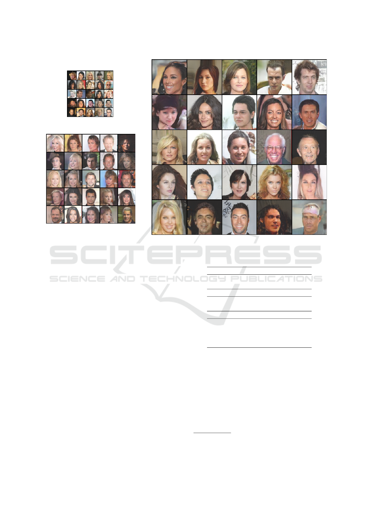
Figure 3: Random generated samples of 32x32, 64x64 and 128x128 resolutions.

extractor. As shown in (Caron et al., 2018), AlexNet

offers an out-of-the-box clustered space at certain

intermediate layer without any need of training.

Hence, we extract there the features and no extra

processing step is involved.

CIFAR10. Despite the fact that CIFAR10 is fairly

close to MNIST in terms of amount of samples and

classes (10 in both cases), it is indeed a much more

complex dataset. As a result, in this case we need to

train a feature extractor to achieve a structured latent

space. Inspired by the unsupervised representation

learning method (Gidaris et al., 2018), we build a

classiﬁer which reaches similar accuracy.

CelebA. Different from the previous datasets, CelebA

contains only ”one class” of images. In particular, this

datatset is an extensive collection of faces. However,

each sample can potentially contain up to 20 different

attributes. So, in our experiments we build different

scenarios by splitting the dataset into different classes

according to their attributes, e.g. man and woman.

Moreover, we also test our approach on different res-

olutions, since the size of the images of CelebA is

larger. Similarly to CIFAR10 case, we need to train

again a feature extractor.

Table 1: Validation results in MNIST, CIFAR10 and

CelebA.

MNIST IS FID Accuracy

baseline 9.63 - -

ours 9.78 - 72%

CIFAR10 IS FID Accuracy

baseline 7.2 28.76 -

ours 7.0 29.71 68%

CelebA IS FID Accuracy

baseline 2.3 18.56 -

ours (32) 2.5 11.10 90%

ours (64) 2.7 13.69 94%

ours (128) 2.65 37.59 94%

4.2 Evaluation Results

We compare the baseline model based on Spectral

Normalization for Generative Adversarial Networks

(SNGAN) (Miyato et al., 2018) to our approach that

incorporates the latent code and the coupled input

on top of it. The rest of the topology remains un-

changed.

We do not use CGAN architecture since

our framework is not conditioned on labels. There-

fore, we take an unsupervised model as a baseline.

In CelebA, we add one and two layers into the model

to be able to produce samples with resolution of 64x64 and

128x128, respectively.

Latent Space Conditioning on Generative Adversarial Networks

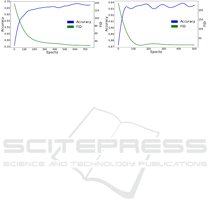
(a) CIFAR10.

(b) CelebA.

Figure 4: FID and accuracy learning curves on CIFAR10 and CelebA.

In particular, we choose SNGAN because it is a sim-

ple yet stable model that allows to control the changes

applied on the system. Besides, it generates appealing

results having a competitive metric scores.

To evaluate generated samples, we report standard

qualitative scores on the Frechet Inception Distance

(FID) and the Inception Score (IS) metrics. Further-

more, we provide the accuracy scores that eventually

quantize the success of the system. We compute this

score using a classiﬁer trained on the real data that

guarantees that the metric correctly assesses the per-

centage of generated samples that coincide with the

class of the latent code. For instance, if the latent code

belongs to a cat, the generator should produce a cat.

Table 1 compares scores for each metric. We ob-

serve how our model performs fairly similar to the

baseline independently of the scenario. Only when

we ask for a 128x128 output resolution, the FID

score increases substantially. We hypothesize that this

break happens due to a model architecture issue since

the baseline is initially designed for 32x32 images

(see Fig. 3). Fig. 4 plots FID and accuracy training

curves on CIFAR10 and CelebA datasets, and con-

ﬁrms that our approach exhibits a strong correlation

between the both metrics. A better FID score (low

value) means always a higher accuracy score.

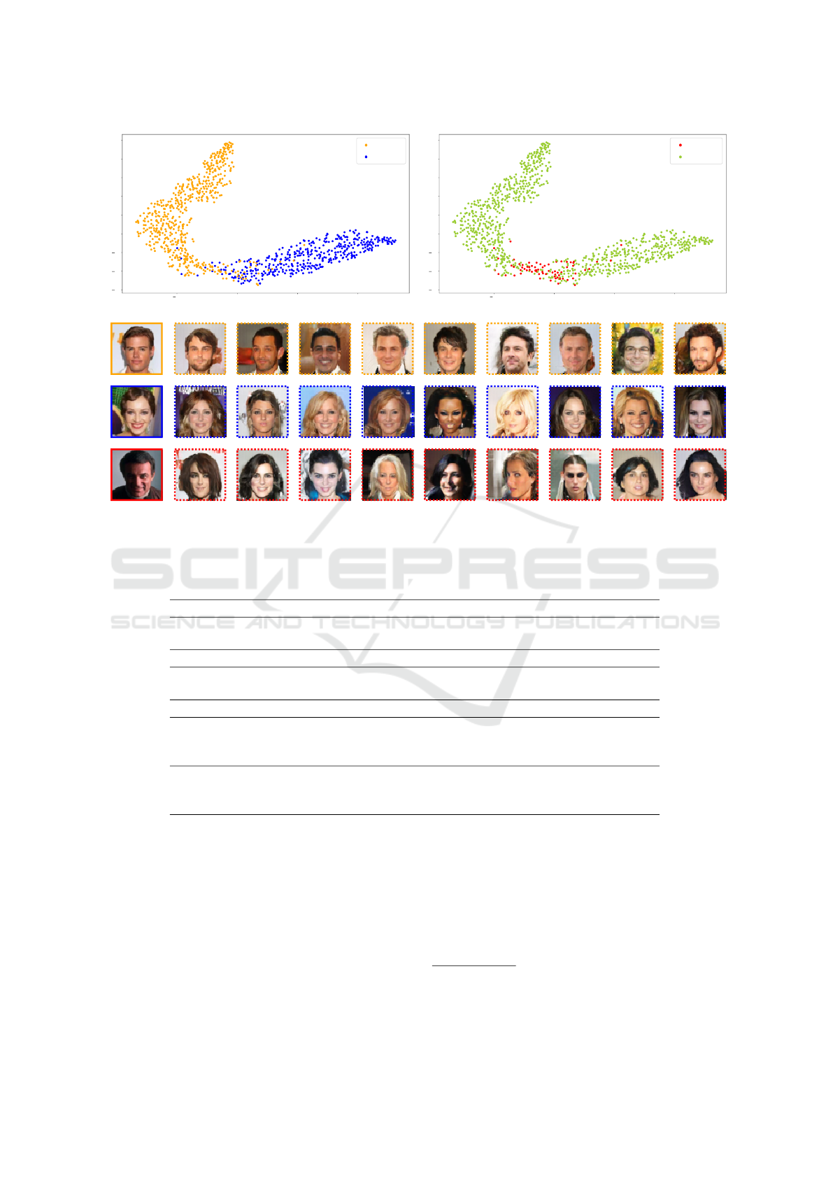
It is important to notice that baseline models do

not have accuracy score since they cannot choose the

class of the output. On the other hand, regarding our

approach, the accuracy for both MNIST and CIFAR is

around 70%, and more than 90% for CelebA. This gap

is directly related with the quality of the latent space.

In other words, the more clustered the latent space

is, the higher accuracy our model can have. In this

case, CelebA is evaluated in a scenario with only two

classes man and women, as a consequence the latent

spaces is simpler. As a rule of thumb, an increase of

classes will often lead to a more tangled latent space

making the problem harder. The main reason for that

are those samples located on the borders. We refer to

this phenomenon as border effect and it is shown in

Fig. 5. As it is expected, we observe how the samples

that lie between the two blobs have usually a higher

failure rate (colored in red).

4.3 Impact of the Latent Space

Structure

The structure of latent space plays an important role

and has a direct effect in the accuracy performance.

This is mainly due to the nature of the triple cou-

pled loss. This term relies on having at least a semi-

clustered feature space to sample from. Hence, those

latent spaces with almost no structure will build many

false couples in training time and resulting in bad

performance. Notice that the generator model does

not use label information directly, but through the ex-

tracted features.

We run the evaluations on MNIST, CIFAR10 and

CelebA datasets as in the previous section. However,

in CelebA’s case there are now two different set-ups.

One based on gender (man and woman), and a sec-

ond one based on hair (blond, black, brown, gray

and bold). In order to study the impact of the latent

space structure, we need to determine how clustered

our space is. Therefore, we compute a set of statistics

(see Table 2) that are useful to estimate the initial con-

ditions of the latent structure, and consequently ﬁnd

out the boundaries that our system might not over-

come. For example, our model on CIFAR10 reports

70% on 1

neighbour. This value indicates that if we

take one random sample from our latent space, 70%

of the time its nearest neighbour will belong to the

same class. Empirically, we observe the causal effect

that the structure of latent space has on the accuracy

results. The more clustered, i.e. higher neighbours

scores, the better the accuracy. In other words, neigh-

bourhood information helps to understand the upper-

bounds ﬁxed by the latent space.

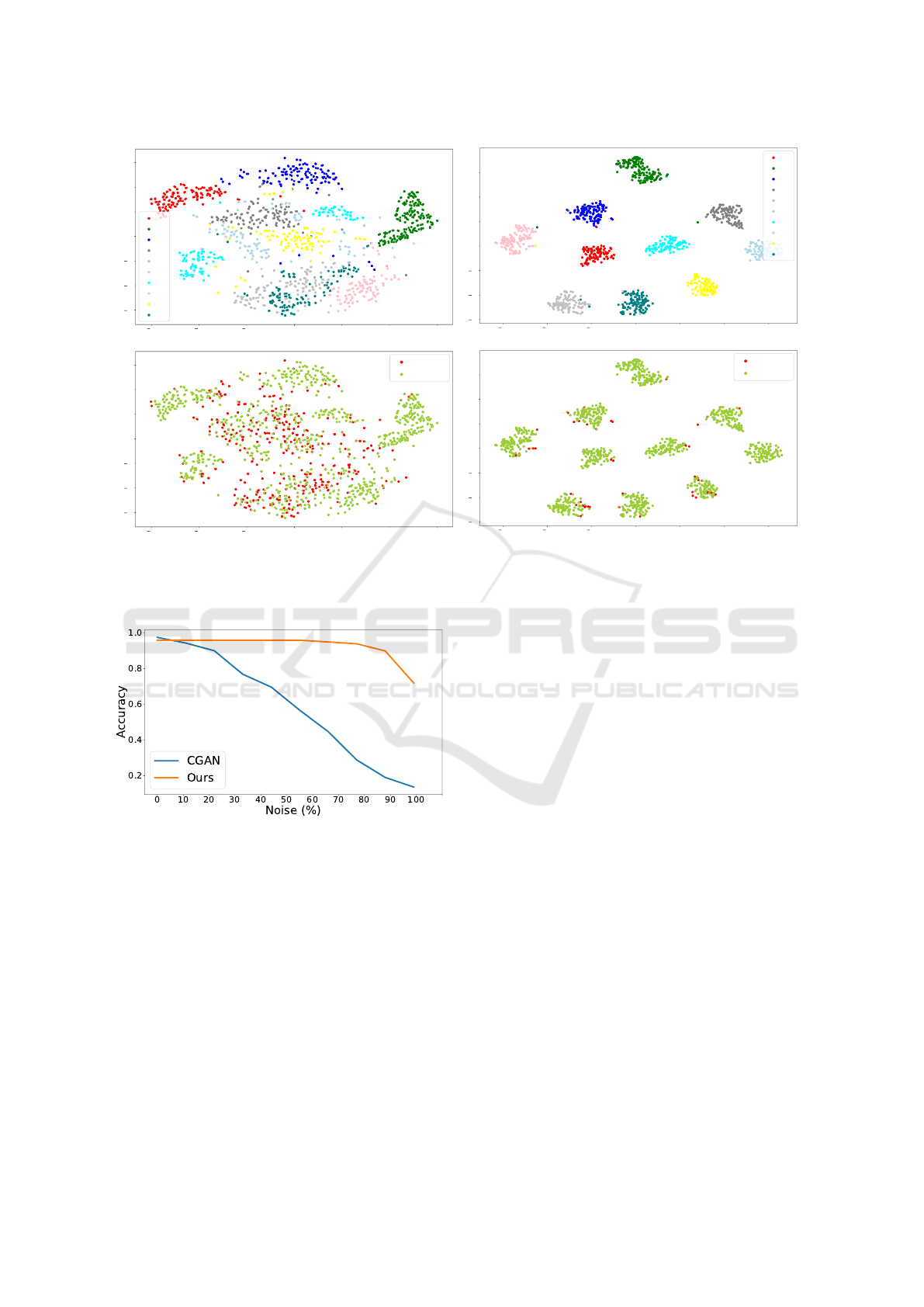
Fig. 6 compares two identical set-ups with differ-

ent latent spaces. On the one hand, we have the semi-

clustered space produced by an untrained AlexNet.

VISAPP 2021 - 16th International Conference on Computer Vision Theory and Applications

20 0 20 40

Dimension 1

Dimension 2

wrong

correct

20 0 20 40

Dimension 1

Dimension 2

man

woman

Figure 5: Visualization of border effect on CelebA for the classes man and woman. Upper-left: t-SNE of extracted features

regarding to their classes. Upper-right: t-SNE of extracted features regarding to their capacity of conditioning the output i.e.

accuracy. Bottom: Random samples from different latent codes, where the solid frame belong to the real images and the

dashed frames the generated. The code color is consistent within the whole ﬁgure.

Table 2: Statistics of the latent space’s structure for different scenarios.

MNIST Classes Accuracy 1

neighbour 2

neighbour 5

neighbour

baseline 10 - 10% 10% 10%

ours 10 72% 89% 84% 78%

CIFAR10 Classes Accuracy 1

neighbour 2

neighbour 5

neighbour

baseline 10 - 10% 10% 10%

ours 10 68% 70% 68% 65%

CelebA Classes Accuracy 1

neighbour 2

neighbour 5

neighbour

baseline 2 - 50% 50% 50%

ours (32) 2 90% 88% 88% 86%

ours (64) 2 94% 95% 94% 93%

baseline 5 - 20% 20% 20%

ours (32) 5 80% 90% 89% 87%

ours (64) 5 78% 96% 95% 92%

This scenario achieves good accuracy scores despite

the border effect. On the other hand, we have an ex-

treme case with a fully-clustered space. As expected,

all the scores are dramatically improved at the cost of

having a perfect space.

4.4 Robustness of the Latent Space

In this section, we analyse how our approach behaves

when we introduce noisy labels, and we compare it

to CGAN performance. This analysis allows us to

quantify how robust our system is. We start the ex-

periments having a set-up free of noise.

Then, we

gradually increase the amount of noise by introduc-

ing noisy labels. Fig. 7 shows the accuracy curves

evolution for both cases. We observe how CGAN has

almost a perfect lineal relationship between noise and

accuracy. Every time that noise increases, the accu-

racy decreases in a similar proportion. This demon-

Notice that for this experiment we take a feature extrac-

tor and we train it from scratch each time that we change the

percentage of noise.

Latent Space Conditioning on Generative Adversarial Networks

60 40 20 0 20 40 60

Dimension 1

Dimension 2

wrong

correct

60 40 20 0 20 40 60

Dimension 1

Dimension 2

(a) Semi-clustered latent space.

60 40 20 0 20 40 60

Dimension 1

Dimension 2

60 40 20 0 20 40 60

Dimension 1

Dimension 2

wrong

correct

(b) Full-clustered latent space.

Figure 6: t-SNE visualizations from two different latent spaces on MNIST. First row displays the classes and second row the

accuracy from our approach.

Figure 7: Robustness evaluation on MNIST using accuracy

curves.

strate the necessity of CGAN of labels to produce the

desired output and the incapacity to deal with noise.

Therefore, its robustness against noise very is limited.

On the other hand, our approach shows a more robust

behaviour. In this case, there is not lineal relationship,

and the system is able to maintain the accuracy score

independently of the level of noise. Only a notable

decrease happens when the percentage of noisy labels

surpasses the barrier of 90%.

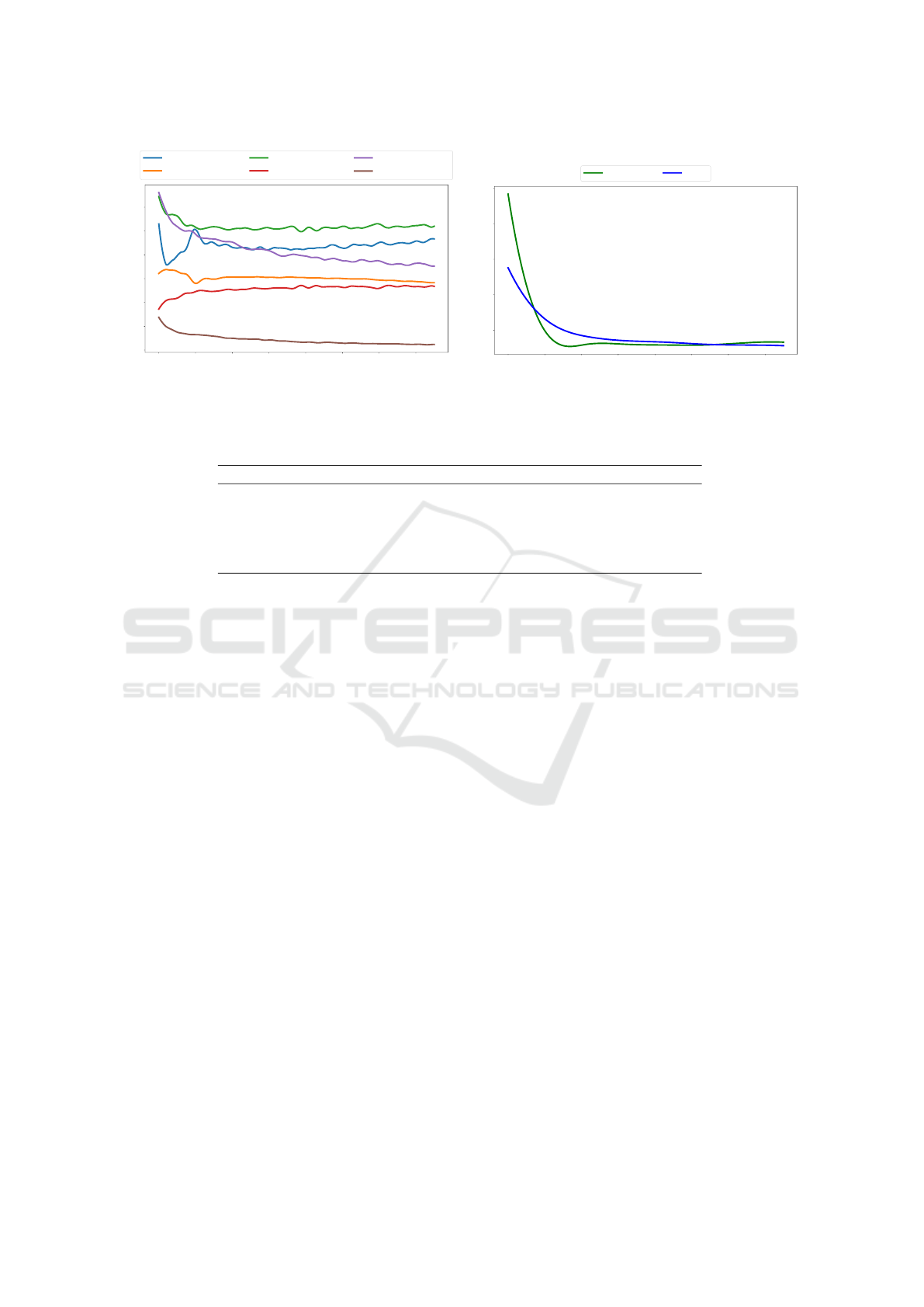
4.5 Analysis of Triple Coupled Loss

The triple coupled loss is designed to exploit the

structure of the latent space, so that the generative

model learns how to produce samples on demand, i.e.

based on the extracted features. Fig. 8 shows the

itemized losses and FID learning curves for minimax

loss (baseline) and for triple coupled loss (ours). We

can conﬁrm a similar behaviour between our model

and the baseline, having as a side-effect an increase

of convergence training time. In exchange for this de-

lay, the proposed system has control over the outputs

through the extracted features.

5 ABLATION STUDY

In this section, we quantitatively evaluate the impact

of removing or replacing parts of the triple coupled

loss. We do not only illustrate the beneﬁts of the

proposed loss compared to minimax loss, but also

present a detailed evaluation of our approach. Table 3

presents how the loss function behaves when we mod-

ify its components. First, we check whether the sub-

optimal loss leads the system to convergence, i.e. it

is able to generate realistic images. And second, for

those functions that have the capacity of generating,

we check their accuracy score. Notice that ideally we

would achieve 100% which means producing the de-

sired output all the time.

Based on the empirical results from the previous

VISAPP 2021 - 16th International Conference on Computer Vision Theory and Applications

0 100 200 300 400 500 600 700

Epochs

0.0

0.2

0.4

0.6

0.8

1.0

1.2

Error

gen (baseline)

disc (baseline)

gen (our)

disc_adv (our)

disc_same (our)

disc_false (our)

(a) Losses evolution.

0 100 200 300 400 500 600 700

Epochs

100

150

200

250

FID

baseline ours

(b) FID evolution.

Figure 8: Comparison between the baseline and our approach on CIFAR10.

Table 3: Quantitative results of the ablation study on CIFAR10.

minimax

adv

same

diff

Convergence Accuracy

baseline X X 8%

prototype A X -

prototype B X X X 58%

prototype C X X -

ours X X X X 68%

table, we can see the importance of each term in the

loss function. In particular, we observe how L

same

essential to achieve convergence, and how the combi-

nation of all three terms brings the best result.

6 CONCLUSIONS

Motivated by the desire to condition GANs without

using label information, in this work, we propose an

unsupervised framework that exploits the latent space

structure to produce samples on demand. In order

to be able to incorporate the features from the given

space, we introduce a new loss function. Our experi-

mental results show the effectiveness of the approach

on different scenarios and its robustness against noisy

labels.

We believe the line of this work opens new av-

enues for feature research, trying to combined differ-

ent unsupervised set-ups with GANs. We hope this

approach can pave the way towards high quality, fully

unsupervised, generative models.

REFERENCES

Aspiras, T. H., Liu, R., and Asari, V. K. (2019). Active re-

call networks for multiperspectivity learning through

shared latent space optimization. In IJCCI, pages

434–443.

Brock, A., Donahue, J., and Simonyan, K. (2018). Large

scale gan training for high ﬁdelity natural image syn-

thesis. arXiv preprint arXiv:1809.11096.

Caron, M., Bojanowski, P., Joulin, A., and Douze, M.

(2018). Deep clustering for unsupervised learning of

visual features. In Proceedings of the European Con-

ference on Computer Vision (ECCV), pages 132–149.

Chen, T., Kornblith, S., Norouzi, M., and Hinton, G. (2020).

A simple framework for contrastive learning of visual

representations. arXiv preprint arXiv:2002.05709.

Chen, T., Zhai, X., Ritter, M., Lucic, M., and Houlsby,

N. (2019). Self-supervised gans via auxiliary rotation

loss. In Proceedings of the IEEE Conference on Com-

puter Vision and Pattern Recognition, pages 12154–

12163.

Chen, X., Duan, Y., Houthooft, R., Schulman, J., Sutskever,

I., and Abbeel, P. (2016). Infogan: Interpretable rep-

resentation learning by information maximizing gen-

erative adversarial nets. In Advances in neural infor-

mation processing systems, pages 2172–2180.

Choi, Y., Choi, M., Kim, M., Ha, J.-W., Kim, S., and Choo,

J. (2018). Stargan: Uniﬁed generative adversarial net-

works for multi-domain image-to-image translation.

In Proceedings of the IEEE conference on computer

vision and pattern recognition, pages 8789–8797.

Chongxuan, L., Xu, T., Zhu, J., and Zhang, B. (2017).

Triple generative adversarial nets. In Advances in neu-

ral information processing systems, pages 4088–4098.

Doersch, C., Gupta, A., and Efros, A. A. (2015). Unsuper-

vised visual representation learning by context predic-

Latent Space Conditioning on Generative Adversarial Networks

tion. In Proceedings of the IEEE International Con-

ference on Computer Vision, pages 1422–1430.

Durall, R., Pfreundt, F.-J., and Keuper, J. (2019). Stabi-

lizing gans with octave convolutions. arXiv preprint

arXiv:1905.12534.

Durall, R., Pfreundt, F.-J., and Keuper, J. (2020). Lo-

cal facial attribute transfer through inpainting. arXiv

preprint arXiv:2002.03040.

Gidaris, S., Singh, P., and Komodakis, N. (2018). Unsu-

pervised representation learning by predicting image

rotations. arXiv preprint arXiv:1803.07728.

Goodfellow, I., Pouget-Abadie, J., Mirza, M., Xu, B.,

Warde-Farley, D., Ozair, S., Courville, A., and Ben-

gio, Y. (2014). Generative adversarial nets. In

Advances in neural information processing systems,

pages 2672–2680.

Gulrajani, I., Ahmed, F., Arjovsky, M., Dumoulin, V., and

Courville, A. C. (2017). Improved training of wasser-

stein gans. In Advances in neural information pro-

cessing systems, pages 5767–5777.

Hinton, G. E. and Roweis, S. T. (2003). Stochastic neigh-

bor embedding. In Advances in neural information

processing systems, pages 857–864.

Hinz, T., Heinrich, S., and Wermter, S. (2019). Generating

multiple objects at spatially distinct locations. arXiv

preprint arXiv:1901.00686.

Ho, K., Keuper, J., and Keuper, M. (2020). Learn-

ing embeddings for image clustering: An empiri-

cal study of triplet loss approaches. arXiv preprint

arXiv:2007.03123.

Hong, S., Yang, D., Choi, J., and Lee, H. (2018). Inferring

semantic layout for hierarchical text-to-image synthe-

sis. In Proceedings of the IEEE Conference on Com-

puter Vision and Pattern Recognition, pages 7986–

7994.

Huang, X., Liu, M.-Y., Belongie, S., and Kautz, J. (2018).

Multimodal unsupervised image-to-image translation.

In Proceedings of the European Conference on Com-

puter Vision (ECCV), pages 172–189.

Isola, P., Zhu, J.-Y., Zhou, T., and Efros, A. A. (2017).

Image-to-image translation with conditional adversar-

ial networks. In Proceedings of the IEEE conference

on computer vision and pattern recognition, pages

1125–1134.

Karras, T., Laine, S., and Aila, T. (2019). A style-based

generator architecture for generative adversarial net-

works. In Proceedings of the IEEE conference on

computer vision and pattern recognition, pages 4401–

4410.

Karras, T., Laine, S., Aittala, M., Hellsten, J., Lehtinen,

J., and Aila, T. (2020). Analyzing and improving

the image quality of stylegan. In Proceedings of the

IEEE/CVF Conference on Computer Vision and Pat-

tern Recognition, pages 8110–8119.

Krizhevsky, A., Sutskever, I., and Hinton, G. E. (2012). Im-

agenet classiﬁcation with deep convolutional neural

networks. In Advances in neural information process-

ing systems, pages 1097–1105.

LeCun, Y., Bottou, L., Bengio, Y., and Haffner, P. (1998).

Gradient-based learning applied to document recogni-

tion. Proceedings of the IEEE, 86(11):2278–2324.

Li, P., Hastie, T. J., and Church, K. W. (2006). Very sparse

random projections. In Proceedings of the 12th ACM

SIGKDD international conference on Knowledge dis-

covery and data mining, pages 287–296.

Liu, Z., Luo, P., Wang, X., and Tang, X. (2015). Deep learn-

ing face attributes in the wild. In Proceedings of In-

ternational Conference on Computer Vision (ICCV).

Mao, Q., Lee, H.-Y., Tseng, H.-Y., Ma, S., and Yang, M.-

H. (2019). Mode seeking generative adversarial net-

works for diverse image synthesis. In Proceedings of

the IEEE Conference on Computer Vision and Pattern

Recognition, pages 1429–1437.

Milbich, T., Ghori, O., Diego, F., and Ommer, B. (2020).

Unsupervised representation learning by discover-

ing reliable image relations. Pattern Recognition,

102:107107.

Mirza, M. and Osindero, S. (2014). Conditional generative

adversarial nets. arXiv preprint arXiv:1411.1784.

Misra, I., Zitnick, C. L., and Hebert, M. (2016). Shufﬂe

and learn: unsupervised learning using temporal order

veriﬁcation. In European Conference on Computer

Vision, pages 527–544. Springer.

Miyato, T., Kataoka, T., Koyama, M., and Yoshida, Y.

(2018). Spectral normalization for generative adver-

sarial networks. arXiv preprint arXiv:1802.05957.

Odena, A., Olah, C., and Shlens, J. (2017). Conditional

image synthesis with auxiliary classiﬁer gans. In Pro-

ceedings of the 34th International Conference on Ma-

chine Learning-Volume 70, pages 2642–2651. JMLR.

org.

Oord, A. v. d., Li, Y., and Vinyals, O. (2018). Representa-

tion learning with contrastive predictive coding. arXiv

preprint arXiv:1807.03748.

Park, T., Liu, M.-Y., Wang, T.-C., and Zhu, J.-Y. (2019).

Semantic image synthesis with spatially-adaptive nor-

malization. In Proceedings of the IEEE Conference

on Computer Vision and Pattern Recognition, pages

2337–2346.

Rao, D., Visin, F., Rusu, A., Pascanu, R., Teh, Y. W., and

Hadsell, R. (2019). Continual unsupervised represen-

tation learning. In Advances in Neural Information

Processing Systems, pages 7647–7657.

Reed, S., Akata, Z., Yan, X., Logeswaran, L., Schiele, B.,

and Lee, H. (2016). Generative adversarial text to im-

age synthesis. arXiv preprint arXiv:1605.05396.

Salimans, T., Goodfellow, I., Zaremba, W., Cheung, V.,

Radford, A., and Chen, X. (2016). Improved tech-

niques for training gans. In Advances in neural infor-

mation processing systems, pages 2234–2242.

Sanchez, E. and Valstar, M. (2018). Triple consistency loss

for pairing distributions in gan-based face synthesis.

arXiv preprint arXiv:1811.03492.

Vincent, P., Larochelle, H., Lajoie, I., Bengio, Y., and

Manzagol, P.-A. (2010). Stacked denoising autoen-

coders: Learning useful representations in a deep net-

work with a local denoising criterion. Journal of ma-

chine learning research, 11(Dec):3371–3408.

Xu, T., Zhang, P., Huang, Q., Zhang, H., Gan, Z., Huang,

X., and He, X. (2018). Attngan: Fine-grained text

to image generation with attentional generative ad-

versarial networks. In Proceedings of the IEEE con-

ference on computer vision and pattern recognition,

pages 1316–1324.

VISAPP 2021 - 16th International Conference on Computer Vision Theory and Applications