
A Surface and Appearance-based Next Best View System for Active
Object Recognition
Pourya Hoseini
a
, Shuvo Kumar Paul
b
, Mircea Nicolescu and Monica Nicolescu
Department of Computer Science and Engineering, University of Nevada, Reno, U.S.A.
Keywords:
Object Recognition, Active Vision, Next Best View, View Planning, Foreshortening, Classification
Dissimilarity, Robotics.
Abstract:
Active vision represents a set of techniques that attempt to incorporate new visual data by employing camera
motion. Object recognition is one of the main areas where active vision can be particularly beneficial. In
cases where recognition is uncertain, new perspectives of an object can help in improving the quality of
observation and potentially the recognition. A key question, however, is from where to look at the object.
Current approaches mostly consider creating an occupancy grid of known object voxels or imagining the
entire object shape and appearance to determine the next camera pose. Another current trend is to show every
possible object view to the vision system during the training time. These methods typically require multiple
observations or considerable training data and time to effectively function. In this paper, a next best view
system is proposed that takes into account only the initial surface shape and appearance of the object, and
subsequently determines the next camera pose. Therefore, it is a single-shot method without the need to have
any specifically made dataset for the training. Experimental validations prove the feasibility of the proposed
method in finding good viewpoints while showing significant improvements in recognition performance.
1 INTRODUCTION
It is a necessity for an intelligent entity to sense its
environment to act informed. One of the main per-
ception mediums is vision. Despite being a heav-
ily used sensing modality, a vision mechanism may
face difficulties in capturing the most useful views
for the specific task at hand. There can be many rea-
sons for such issues, including occlusion, lack of dis-
criminative features due to bad lighting or unfavor-
able viewpoints of the object, or insufficient image
resolution. Active vision is an answer to those situa-
tions that tries to enhance the performance of the vi-
sion system by dynamically incorporating new visual
sensory sources. Some application domains of active
vision are three-dimensional (3D) object reconstruc-
tion and object recognition, the latter being the focus
of our work. Active Object Recognition (AOR) has
many uses in robotics (Paul et al., 2020), vision-based
surveillance, etc. AOR procedures normally involve
uncertainty evaluation, camera movement, matching,
and information fusion (Hoseini et al., 2019a) and
(Hoseini et al., 2019b). If the current recognition is
a
https://orcid.org/0000-0003-3473-9906
b
https://orcid.org/0000-0003-1791-3925
not certain enough, a camera is moved to observe the
object from another viewpoint and to fuse the current
and new information, usually classification decisions,
from the matched objects in the views, in order to ob-
tain improved results.
Regarding the camera movement, a primary ques-
tion to answer is where and in what orientation a
camera should be placed to fetch the next best view
(NBV) of the object. Finding next best view is an
ill-posed task, because the current viewpoint of the
object is usually not sufficient to deterministically de-
duce the object shape and appearance from its other
facets. Approaches to NBV are generally impacted
by the specific application they are being employed
for. In 3D reconstruction applications, a NBV that
plans to acquire a chain of views that are aimed to ex-
plore unobserved voxels of objects might be an ideal
option. In contrast, the next views in an object recog-
nition application are desired to present new discrim-
inative features, by which the object recognition per-
formance can be enhanced. The number of planned
views for object recognition is also intended to be as
low as possible to reduce energy and time spent mov-
ing the cameras physically.
A deep belief network is presented in (Wu et al.,
2015) to “hallucinate” the whole object shape and ap-
pearance in the presence of occlusion to compute the
recognition uncertainty in several predefined camera
poses. The viewpoint with the least uncertainty is
then selected. Although interesting, this idea has a
major flaw in depending heavily on the estimation of
the object shape and appearance, which can be a large
source of errors. In contrary to (Wu et al., 2015), the
work in (Doumanoglou et al., 2016) directly estimates
the classification probabilities of different views in-
stead of rendering their hypothetical object appear-
ances to compute the information gain in each view.
Despite overcoming the problem of computationally
expensive renderings of hypothetical 3D objects, this
approach requires 3D training data for every test ob-
ject and performing classification and confidence es-
timation for every viewpoint of the 3D objects in the
training. This prerequisite significantly affects the
functionality of the technique due to the scarcity of
such training data for many real-world objects.
A boosting technique is proposed in (Jia et al.,
2010) to combine three criteria for determining the
NBV around objects. The first criterion compares
the similarity of the current object with prerecorded
object appearances in different views and selects the
one with the least similarity. The other two crite-
ria for choosing NBV are the prior probability of a
viewpoint in successfully determining the object class
given either a currently detected object pose or a cur-
rently detected object category. Aside from the priors,
which are application data specific, using a similarity
measure between the current viewpoint of an object
and its other viewpoints requires a dataset made of
images around the training objects with their known
pose. This can be practically burdensome as there is a
need to capture poses and appearances all around the
objects that are to be detected at test time.
Rearranging depth camera positions based on imi-
tating barn owls’ head motions is examined in (Barzi-
lay et al., 2017) for 3D reconstruction of objects. The
method in (Barzilay et al., 2017) mimics motions re-
gardless of the object shape and appearance, which
can cause missing some important clues in determin-
ing the next best view. In (Atanasov et al., 2014),
an active pose estimation and object detection frame-
work is described to balance the odds of object detec-
tion enhancement and the energy needed to move the
camera. A multitude of captures are planned along the
fastest way the camera is moved toward the object.
Since the active vision system of (Atanasov et al.,
2014) does not consider the object shape and appear-
ance and merely moves the camera towards an object,
it cannot be deemed as an intelligent viewpoint selec-
tion method.
A trajectory planning technique for an eye-in-
hand vision system on a PR2 robot is presented
in (Potthast and Sukhatme, 2011) to boost the ex-
pected number of voxel observation by searching for
maximum local information gain. In continuation
to the work of (Potthast and Sukhatme, 2011), a
next best view method for 3D reconstruction applica-
tions on the basis of predicting information gain from
prospective viewpoints is proposed in (Potthast and
Sukhatme, 2014). To predict the information gain in
unobserved areas, an occupancy grid is formed out
of all the observations so far, and a Hidden Markov
Model (HMM) is used to estimate the observation
probability of unobserved cells in the grid.
By reviewing the literature, we see that the earlier
work in determining the next best view is clustered
in two groups: space occupancy-based and object
estimation-based techniques. Assessing occupancy of
3D space via ray tracing and computation of informa-
tion gain is intrinsically beneficial for 3D reconstruc-
tion purposes, because it attempts to discover more
surface voxels than discriminative features for classi-
fication. That is why it has been preferred regularly in
previous work for 3D reconstruction. In contrast, ob-
ject estimation techniques depend on either “halluci-
nating” the 3D shape of the current object or compar-
ing the current object shape and/or appearance to the
ones acquired during training to infer the best camera
pose by comparing different viewpoints. Their prob-
lem is, however, the reliance on large datasets of ob-
ject images taken from predefined points of view as
well as in the inaccuracies stemming from hypotheti-
cal object shapes/appearances.
In this paper, a single-shot next best view method
for object recognition tasks is presented, which plans
for one new viewpoint based on cues from the cur-
rently visible object shape and appearance to improve
the object recognition performance when necessary.
The proposed NBV method is neither reliant on a
prior dataset of specifically designated images from
around the object, nor on 3D object volumes for train-
ing. It uses conventional datasets, a collection of ran-
dom images of objects, merely for the training of the
classifiers. It also does not involve a chain of cam-
era motions toward or around the object to save time
and energy for camera motion. To achieve these char-
acteristics, an ensemble of criteria is used to analyze
different areas of the current view for appearance and
shape cues to suggest a new camera pose. Exam-
ples of such criteria are classification dissimilarity be-
tween a region of the object image and the whole
image, foreshortening, and various statistical texture
metrics. A test dataset was also created to evaluate
the proposed method in a systematic way. In the tests,
the proposed NBV system confirms its efficacy in pre-
dicting the next best camera view among a set of pre-
selected test-time poses around the object. The main
contributions of the proposed work are:
1. A novel next best system is proposed exclusively
for the task of object recognition.
2. The current object shape and appearance are only
used in the proposed NBV; hence no prior knowl-
edge of objects is needed.
3. There is no need to create specially designed
datasets for the next best view determination. The
only training employed is for the object classi-
fiers.
4. A small test dataset, comprised of the images cap-
tured around various objects, has been gathered to
efficiently test the proposed NBV system. It can
be used by other researchers as a benchmark.
5. Experimental validation shows good results in
terms of the performance improvement after fu-
sion of views among a pre-defined set of possible
camera poses.
The remainder of the paper is organized as fol-
lows. The proposed next best view system is pre-
sented in section 2. Section 3 shows the results ob-
tained in the benchmarks. Lastly, concluding remarks
are discussed in section 4.
2 THE PROPOSED SINGLE-SHOT
NEXT BEST VIEW METHOD
In order to find a candidate viewpoint in a single try
after the initial capture, only the color and depth in-
formation of the initial camera view are assumed to
be available. For rigorous testing purposes, the NBV
poses are restricted to a number of pre-specified poses
that are typically reachable for eye-in-hand or UAV
platforms. The poses around any object are clustered
into eight groups in the current implementation, all of
them on the plane that passes through the object and
is parallel to the image plane of the camera at the ini-
tial viewpoint. Each group is the set of poses that are
generally viewing the same part of the object.
The viewpoints are selected to be at the same
depth as the object in the camera coordinate of the
initial view, because they can provide substantially
new information from a view direction perpendicular
to the initial one, but still are reasonably accessible
for many eye-in-hand arrangements. Any pose from
a depth less than the object’s depth will probably see
common parts of the object as the frontal initial view.
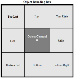
Figure 1: Tiling routine in the proposed next best view sys-
tem.
In contrast, any pose with a depth farther than the ob-
ject will see behind the object, which can be desirable,
but has two disadvantages. First, it is hard to reach by
a robotic system. Many robotic arms do not have the
degrees of freedom required to move an arm-mounted
camera to a pose facing the back of the object, as well
as to poses at a large distance from the robot. It is also
challenging to plan for a pose behind an object for a
freely moving camera unit as the object’s thickness is
unknown in a single frontal shot. The second reason
is that for a single NBV based on the current frontal
view of an object, we are not aware of the worthiness
of the self-occluded area behind the object for active
object recognition camera poses. Therefore, the op-
tion of seeing behind an object is not considered as a
candidate for a next viewpoint.
2.1 Local Analysis of the Current View
In the proposed method, the object bounding box,
emerging from any object detection system, is divided
into different regions. The tiled regions cover the en-
tire area of the bounding box in a non-overlapping
fashion. Figure 1 illustrates the tiling scheme in the
proposed method. Each bounding box is divided into
nine regions in the current implementation, where
each of the eight peripheral tiles corresponds to one of
the pose groups of a camera around the object. For in-
stance, the top left tile represents a point of view when
the camera is viewing the object from the object’s top
left with the same depth to the camera as the object
itself in the camera coordinate of the initial view. The
camera in the new orientation can be placed arbitrar-
ily close to the object considering the pose feasibility
for the camera setup and the image resolution of the
camera. Figure 2 shows this example situation.
The rationale behind this tiling scheme is that an-
alyzing each region of the current view can reveal
clues to a more informative NBV corresponding to
the side of the object it is representing. In con-
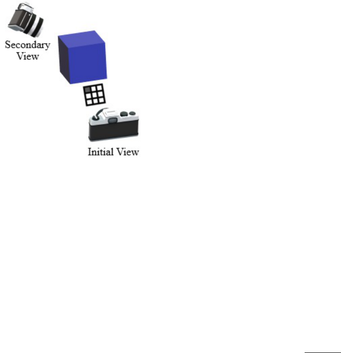
Figure 2: An example next viewpoint selection situation,
where the top left tile is selected and consequently the sec-
ondary viewpoint is looking at the object from its top left.
trast to methods of (Potthast and Sukhatme, 2011),
(Potthast and Sukhatme, 2014), (Doumanoglou et al.,
2016), (Rebull Mestres, 2017), (Krainin et al., 2011),
and (Bircher et al., 2016) that simply attempt to
look at unobserved voxels, the proposed approach
tries to further qualify its decision based on what
is currently being seen. Additionally, the proposed
method differs from techniques of (Wu et al., 2015)
and (Doumanoglou et al., 2016) that hypothesize
the object shape, as it only utilizes limited cues di-
rectly available in the initial view, instead of requiring
the inference of explicit information about the entire
shape, appearance, and relative pose of the object.
2.2 The Ensemble of Viewpoint Criteria
In the proposed method an equally weighted voting
mechanism among four criteria selects the peripheral
tile with the highest votes. Only a single vote is cast
for the tile with the highest score from each criterion.
Two of the criteria statistically analyze the texture of
a tile. Another one evaluates the foreshortening of the
object to estimate how visible its surface was in the
initial view. The last criterion considers the classifi-
cation dissimilarity between a tile and the entire ob-
ject. In the following three subsections, we explain in
detail the 4 voting criteria.
2.3 Statistical Texture Metrics
One of the instances where active vision proves to
be helpful is when the object being observed is not
clearly recognizable due to occlusion, lighting condi-
tions, object shape, etc. One way to confront these
situations can be to shift the view toward poses that
are likely to be well-lit and provide better quality im-
ages. To this end, the second and third moment tex-
ture analysis tools are utilized. The two criteria are
chosen to be obtained from the intensity histograms
of each tile’s image to help in their faster processing.
2.3.1 Second Moment (Variance) of Histogram
A high-contrast image has a higher chance of con-
taining more features than a uniform one. The second
moment or variance of intensity histogram is a mea-
sure of contrast of an image (Gonzalez, 2018). The
variance of an intensity histogram is defined in (1)
(Gonzalez, 2018).
σ
2
(z) = µ
2
(z) =
L−1
∑
i=0
(z
i
− m)
2
p(z
i
) (1)
In the equation, σ
2
(z) is the variance of intensity
levels (z), which is identical to the second moment,
µ
2
(z). In Addition, L represents the total number of
intensity levels in the histogram, i is the index of the
current intensity level, p(z
i
) is the probability of an
intensity level, and m is the mean of intensities, com-
puted as follows:
m =
L−1
∑
i=0
z
i
p(z
i
) (2)
To scale the metric to the range of [0, 1), the con-
trast score V (z) is calculated via (3).
V (z) = 1 −
1
1 + σ
2
(z)
(3)
The scaled second moment, V (z), should be high
ideally, because a greater V(z) means higher contrast
and perhaps more features, with which a tile can be a
cue to a feature-rich sideward surface for a good next
viewpoint.
2.3.2 Third Moment of Histogram
The third moment can be used as a way to measure
how skewed is a histogram towards dark or bright lev-
els (Gonzalez, 2018). It is defined in (4).
µ
3
(z) =
L−1
∑
i=0
(z
i
− m)
3
p(z
i
) (4)
A positive µ
3
(z) indicates a histogram with more
probable bright intensity levels. A histogram weigh-
ing more towards darker intensities is also expected
with a negative third moment. Therefore, to find a
well-lit surface that is neither bright nor dark, we can
seek for a third moment close to zero. Good light-
ing in a boundary tile may signal the existence of the

same condition for the corresponding side of the ob-
ject, which is desirable. Equation (5) is introduced
in the following to translate preferable lighting condi-
tions to a higher score. In (5), higher L(z) values are
related to close to zero third moments, while lower
L(z) can be a result of large or small third moments.
L(z) =
1
1 +
|
µ
3
(z)
|
(5)
2.4 Foreshortening Score
Considering that we examine all criteria on the pe-
riphery tiles of an object’s bounding box, an object
surface with less foreshortening probably means that
it should be easily visible to the sensor in a peripheral
tile. However, in that case, since the peripheral sur-
face has less perspective to the camera’s image plane
and its plane is on average closer to being parallel to
the camera, there should be other faces of the object
that are not being viewed by the camera. On the other
hand, a peripheral surface with a perspective to the
current view, is likely not clearly visible in the current
view as its surface is tilted and exhibits foreshorten-
ing too. Based on this idea, the foreshortening score
considers how much foreshortening is present, or in
other words how parallel is the object surface being
seen in a tile to the image plane of the 3D camera ob-
serving the object. Assuming the depth map of a tile
is segmented, and the object surface constitutes the
foreground pixels, the foreshortening score is defined
in the following:
P = −
∑
p∈F
N
−−−−−−−→
(
dz
dx
p
,
dz
dy
p
, 1)
.
−→
z
|
F
|
(6)
where P is the foreshortening score, p is a pixel in
the current tile, F is the set of foreground pixels,
|
F
|
shows the number of pixels in the tile that are desig-
nated as foreground, N() stands for a function to nor-
malize a vector, and
−→
z is the depth axis in the initial
view’s camera coordinate. The derivatives of depth
(z) with respect to x and y axes in the initial view’s
pixel coordinate are calculated for a particular pixel
(x
p
, y
p
) in the following way:
dz
dx
x=x
p
= z(x
p
+ 1, y
p
) − z(x
p
− 1, y
p
) (7)
dz
dy
y=y
p
= z(x
p
, y
p
+ 1) − z(x
p
, y
p
− 1) (8)
The z(., .) in (7) and (8) signifies the depth at a
pixel of the depth map. To obtain a depth map, the
initial viewpoint must be captured by a 3D camera. It
is common for ordinary 3D cameras to produce small
fragments of unknown values spread over their gener-
ated depth map. To resolve this issue, the maximum
depth in the current tile is replaced over all the un-
known values. We are assuming that large depth val-
ues are attributed to the background. To eliminate the
background from affecting the score, only the fore-
ground areas (F) obtained through Otsu’s segmenta-
tion (Otsu, 1979) are used in (6).
For every foreground pixel in the depth map the
term N(
−−−−−−−→
(
dz
dx
p
,
dz
dy
p
, 1)) in (6) computes the normalized
surface normal. The inner product of the surface nor-
mal and the z axis of the camera coordinate mea-
sures how parallel are the object surface and the im-
age plane of the camera in the initial view, effectively
quantifying the foreshortening of the object. Ulti-
mately, to find the average parallelism of the object
surface to the camera, the results of the inner prod-
ucts are averaged over all the foreground pixels. The
proposed score prefers a tile when its score is higher.
2.5 Tile Classification Dissimilarity
When an AOR system is uncertain about its recogni-
tion, it can be a good idea to find where in the initial
view (i.e. which tile) is contributing more to the un-
certainty by not confirming the initial view’s recogni-
tion. Later, trying to take a new look from the direc-
tion of that opposing tile will probably help in getting
new information and resolving the ambiguity. Ac-
cordingly, to measure the extent of dissimilarity of
class probabilities of the whole object image and a
tile, the sum of their absolute differences (SAD) is
used. This criterion is defined in (9).
S
j
=
∑
i∈G
p
c
j
t
j
(i) − p
c
o
(i)
(9)
where S
j
is the dissimilarity score between the tile j
and the complete object image, G represents the set of
object classes, and p
c
j
t
j
(i) and p
c
o
(i) are probabilities
of a class i after classifying the tile j and the whole
object image by the classifiers trained for tile j (c
j
)
and the whole object (c), respectively. The c and c
j
are conventional classifiers, trained with color images
of objects, with the difference that c
j
only uses the
portion of images related to tile j, while c considers
the whole object images in the training.
3 EXPERIMENTAL RESULTS
The proposed next best view method was evaluated on
a dataset we created, particularly for benchmarking of
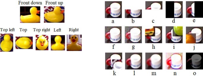
Figure 3: A sample situation in the dataset.
active object recognition techniques. To produce un-
certain initial recognitions that cause an active object
recognition system to trigger, the initial views of ob-
jects were intentionally distorted in the tests. In addi-
tion, the tests were performed on AOR systems with
different classifiers and fusion methods to ensure the
results are not biased for a specific type of AOR sys-
tem.
3.1 The Test Dataset for Active Object
Recognition
We collected 240 test situations, generally for evalu-
ating active recognition systems, especially next best
view methods. The dataset is comprised of 10 ob-
jects, each one being shown in 24 situations. The ob-
jects in each of their 24 test situations were placed in
various poses (4 random faces of the object), lighting
conditions (2 modes: darker and brighter), and back-
ground textures (3 modes: dark tabletop, light carpet,
and colorful rug). There are seven images and their
corresponding depth maps in each situation: one for a
frontal initial view, another for an initial view with a
slightly higher altitude initial view, and five others for
the images/depth maps taken from the sides of objects
as follows: left, top left, top, top right, and right. Fig-
ure 3 shows a sample situation for one of the objects
in the dataset. The dataset is published along with the
current paper.
3.2 Emulating AOR Triggering
Conditions
Active object recognition systems are normally used
when the classifiers suffer reduced performance due
to occlusion or unfavorable perspective of objects.
Because the initial views in the test dataset are clear
and unobstructed, the initial views are altered to cre-
ate the conditions that can trigger AOR. These alter-
ations are superimposing a corner of the image and its
respective depth map, amounting to 36% of their area,
by a patch of another randomly selected object image
Figure 4: Initial view distortions. a) Original im-
age, b, c) Top/bottom whiteout, d, e) Left/right blackout,
f, g) Lighter/heavier noise, h, i, j, k) Corner superimpose,
l, m) Lighter/heavier blur, n) Bright, o) Dark.
and its depth map, replacing with white or black an
entire half of the image and its corresponding depth
map, Gaussian blurring in two levels, adding noise in
two levels, and image brightening/darkening.
The tests were performed on the original images
and their altered versions as well as their correspond-
ing depth maps, totaling 15 test scenarios for any test
situation in the dataset. Figure 4 shows the 15 ver-
sions of the initial view for an object in a sample situ-
ation.
3.3 Test Benchmarks
Since there are two initial images in each test situation
in the dataset, two experiments can be performed for a
single situation. As mentioned in the former section,
for each initial image 15 test scenarios with various
alterations are possible. Therefore, 30 tests are per-
formed for any test situation. With the existence of
240 test situations in the dataset, 7200 situations were
evaluated for any vision system in the tests.
To ensure that the proposed NBV is independent of
the classifier and the fusion algorithms in the AOR
system, five different classifiers and three fusion tech-
niques were examined in order to take their aver-
age results. Averaging, Na
¨
ıve Bayes (Hoseini et al.,
2019a), and Dempster-Shafer (DS) (Hoseini et al.,
2019b) fusion algorithms are used in the tests. Three
of the classifiers are Convolutional Neural Network
(CNN) models with different number and composi-
tion of layers, activation functions, and pooling op-
erations. Another one is a Support Vector Machine
(SVM) classifier with the feature vector comprised
of Hu moments of the three RGB (red-green-blue)
planes, besides the reduced Histogram of Oriented
Gradients (HOG) of the gray level image of the in-
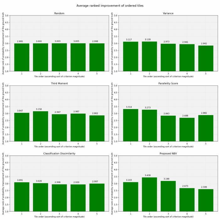
Figure 5: Average ranked improvement of tiles in ascending order of scores.
put. The last one is a random forest that uses a bag of
visual words of Speeded Up Robust Features (SURF)
keypoint descriptors.
Considering the possible combinations of the classi-
fication and fusion approaches, 15 benchmarks were
evaluated, each with 7200 situations tested. In the
tests, the confidence threshold of the AOR, explained
in (Hoseini et al., 2019a) and (Hoseini et al., 2019b),
was set to 20, that means the second viewpoint is re-
trieved if the highest class probability of the initial
view is less than 20 times of the second highest one.
3.4 Obtained Results
3.4.1 Ranked Ground Truth Improvement
In every test situation, the five prospective next view-
points are examined for the scores they get from every
criterion. In Figure 5, the tiles are sorted on the hori-
zontal axis in an ascending order of the scores of each
designated criterion. The height of the bars for any
tile shows the mean rank of the tile in attaining better
probability for the ground truth classes after the deci-
sion fusion stage. The lower the rank and the closer
it is to 1, the better it is. Therefore, in Figure 5 it is
desirable to have lower height of the bars in the right
sides of the plots.
From the results, it can be seen that the proposed
NBV method attains better ranks for the tiles it scores
higher. It means that it is useful in selecting the view-
points that offer the best improvement in probability
of the true class in the AOR system’s output. Addi-
tionally, Figure 5 shows the performance of randomly
selecting the next view and the individual criteria that
are part of the ensemble. All the proposed individ-
ual criteria in the ensemble mostly find the better tiles
with their scorings and tend to bring the height of their
very right bar down, despite being not as good as the
combination of them, which causes sharper decline in
the height of the right bar.
3.4.2 Performance per Criterion
Figure 6 compares the ratio of accuracy, precision, re-
call, and F
1
score improvement of the proposed sys-
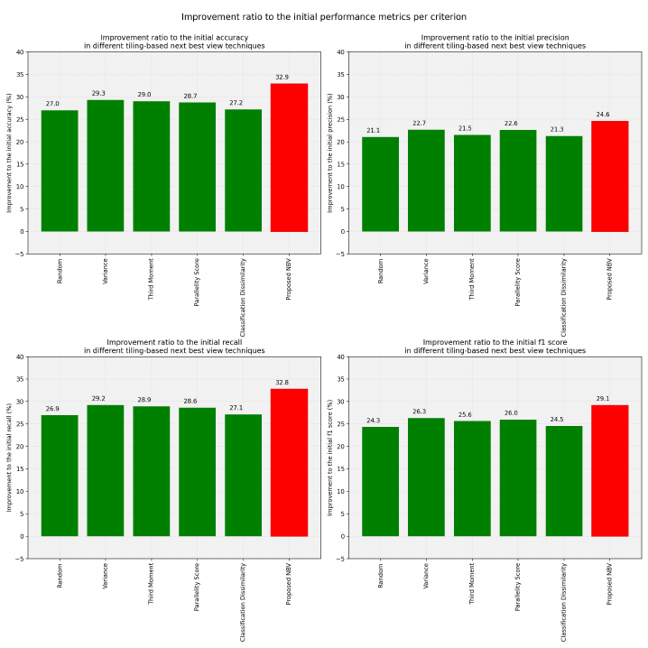
Figure 6: Improvement ratio to the initial performance metrics per measure.
tem and its constituting measures as well as random
view selection to their initial performance metrics.
We see that the proposed system achieves high im-
provements and is better than the other criteria in the
figure, including the random selection of next view-
point. Accuracy and F
1
score of the proposed method
is 5.9% and 4.8% more than a randomly viewpoint
selecting AOR system.
3.4.3 Performance Improvement per Sorted
Tiles
The accuracy, precision, recall, and F
1
score improve-
ment of the AOR system by using any of the five pos-
sible tiles in the tests are shown in Figure 7. The tiles
are sorted in the horizontal axis based on the scores
they receive from each measure. It is desirable to see
better performance for the tiles the NBV system em-
phasizes more, i.e. the ones with higher scores in the
right side of each plot. Therefore, we want to see
higher bars on the right side of each plot. The re-
sults prove that the proposed NBV is effective in ob-
taining higher performance indices in its top picks.
The individual measures participating in the ensem-
ble also show a trend of increasing accuracy, preci-
sion, recall, and F
1
score with the higher scores they
produce, which is not always true for the random se-
lection.
3.4.4 Receiver Operating Characteristic (ROC)
Curves
Figure 8 shows the ROC curves obtained through
micro-averaging for all the samples in the 15 bench-
marks. The blue curves in the figure, show the re-
sults of the initial view recognitions only, while the
green curves indicate the effect of fusing with the re-
sults of a randomly selected view. The red curves,
instead, show the results of utilizing the proposed
method. Comparing the three sets of the curves veri-
fies the effectiveness of the AOR system in enhancing
the ROC curve, and of the NBV method in increasing
the recognition improvement.
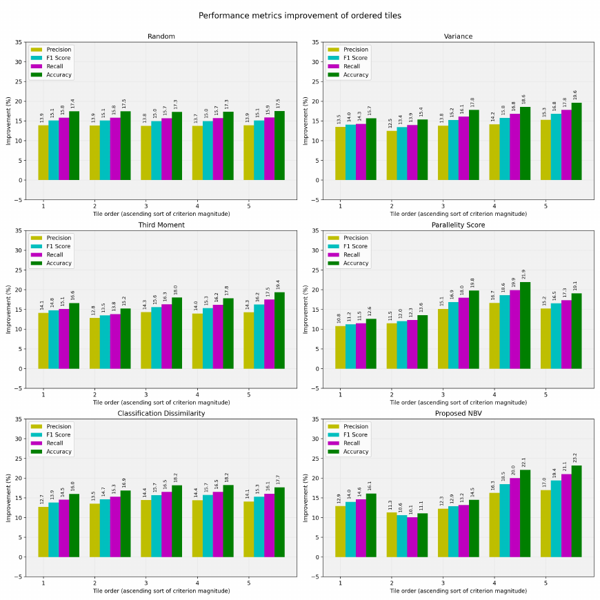
Figure 7: Performance metrics improvement of tiles in ascending order of scores.
3.5 Discussion
The experimental results clearly show the applicabil-
ity of the proposed NBV in improving accuracy, re-
call, precision, and thus F
1
score of the active object
recognition systems. In the results, we observe that
the active object recognition systems with a random
selection of next viewpoint attain 27% and 24.3% ac-
curacy and F
1
score improvement on average. With
the proposed next best view method, the same AOR
systems experience 32.9% and 29.1% accuracy and
F
1
score enhancements, which amounts for 5.9% and
4.8% further improvement over a random AOR.
Interestingly, the tile ranking using the foreshortening
score shows that sometimes the tiles with the penul-
timate score reach better ranks than the highest scor-
ing ones. Those cases occur perhaps when the higher
scoring tile has a very steep object surface with re-
spect to the image plane of the camera in the initial
view. Compared to less steep surfaces, a very steep
one may impede the proper view of the respective ob-
ject side from the perspective of the initial view.
4 CONCLUSION
In this paper a next best view approach for active ob-
ject recognition systems was presented. The proposed
view selection divides an initial image of an object
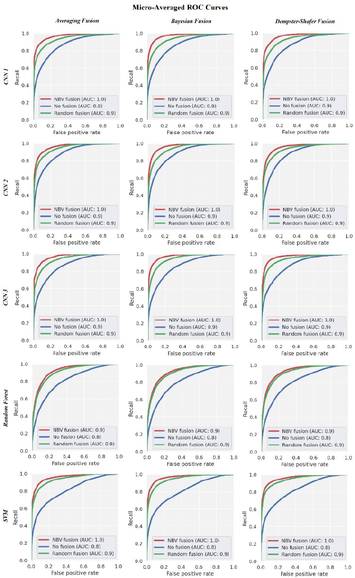
Figure 8: ROC curves of different test benchmarks.
into a few zones to investigate each one for clues in
determining better next views. Each area is analyzed
through an ensemble of four different techniques:
foreshortening, histogram variance, histogram third
moment, and classification dissimilarity. There is no
need to a prior training set of specific views of ob-
jects or their 3D models in the proposed method. It
can suggest the next viewpoint based on just the in-
formation of a single initial view, which along with
the property of considering both the 3D shape and ap-
pearance of objects offers an intrinsic advantage for
active object recognition tasks.
A dataset for testing active object recognition systems
was developed as a part of this work and was used to
evaluate the proposed next best view technique. In
the presence of heavy occlusions in the initial view,
we report 32.9% and 29.1% average accuracy and F
1
score improvements compared to the initial perfor-
mance values.
In continuation to this work, future efforts should be
directed toward probing alternative tiling schemes of
the initial view. Another area of work can be investi-
gating other ensemble methods in place of the current
voting scheme. A meta-learning approach would be a
potentially interesting way to combine the tile scores.
ACKNOWLEDGMENTS
This work has been supported in part by the Office
of Naval Research award N00014-16-1-2312 and US
Army Research Laboratory (ARO) award W911NF-
20-2-0084.
REFERENCES
Atanasov, N., Sankaran, B., Le Ny, J., Pappas, G. J., and
Daniilidis, K. (2014). Nonmyopic view planning for
active object classification and pose estimation. IEEE
Transactions on Robotics, 30(5):1078–1090.
Barzilay, O., Zelnik-Manor, L., Gutfreund, Y., Wagner, H.,
and Wolf, A. (2017). From biokinematics to a robotic
active vision system. Bioinspiration & Biomimetics,
12(5):056004.
Bircher, A., Kamel, M., Alexis, K., Oleynikova, H., and
Siegwart, R. (2016). Receding horizon” next-best-
view” planner for 3d exploration. In 2016 IEEE in-
ternational conference on robotics and automation
(ICRA), pages 1462–1468. IEEE.
Doumanoglou, A., Kouskouridas, R., Malassiotis, S., and
Kim, T.-K. (2016). Recovering 6d object pose and
predicting next-best-view in the crowd. In Proceed-
ings of the IEEE conference on computer vision and
pattern recognition, pages 3583–3592.
Gonzalez, R. C. (2018). Richard E. Woods Digital Image
Processing, Pearson. Prentice Hall.
Hoseini, P., Blankenburg, J., Nicolescu, M., Nicolescu, M.,
and Feil-Seifer, D. (2019a). Active eye-in-hand data
management to improve the robotic object detection
performance. Computers, 8(4):71.
Hoseini, P., Blankenburg, J., Nicolescu, M., Nicolescu, M.,
and Feil-Seifer, D. (2019b). An active robotic vi-
sion system with a pair of moving and stationary cam-
eras. In International Symposium on Visual Comput-
ing, pages 184–195. Springer.
Jia, Z., Chang, Y.-J., and Chen, T. (2010). A general
boosting-based framework for active object recogni-
tion. In British Machine Vision Conference (BMVC),
pages 1–11. Citeseer.
Krainin, M., Curless, B., and Fox, D. (2011). Autonomous
generation of complete 3d object models using next
best view manipulation planning. In 2011 IEEE In-
ternational Conference on Robotics and Automation,
pages 5031–5037. IEEE.
Otsu, N. (1979). A threshold selection method from gray-
level histograms. IEEE transactions on systems, man,
and cybernetics, 9(1):62–66.
Paul, S. K., Chowdhury, M. T., Nicolescu, M., Nicolescu,
M., and Feil-Seifer, D. (2020). Object detection and
pose estimation from rgb and depth data for real-time,
adaptive robotic grasping. In 24th International Con-
ference on Image Processing, Computer Vision, &
Pattern Recognition (IPCV). Springer.
Potthast, C. and Sukhatme, G. S. (2011). Next best view
estimation with eye in hand camera. In IEEE/RSJ Intl.
Conf. on Intelligent Robots and Systems (IROS). Cite-
seer.
Potthast, C. and Sukhatme, G. S. (2014). A probabilistic
framework for next best view estimation in a cluttered
environment. Journal of Visual Communication and
Image Representation, 25(1):148–164.
Rebull Mestres, J. (2017). Implementation of an automated
eye-in hand scanning system using best-path planning.
Master’s thesis, Universitat Polit
`
ecnica de Catalunya.
Wu, Z., Song, S., Khosla, A., Yu, F., Zhang, L., Tang, X.,
and Xiao, J. (2015). 3d shapenets: A deep representa-
tion for volumetric shapes. In Proceedings of the IEEE
conference on computer vision and pattern recogni-
tion, pages 1912–1920.
