Variation-resistant Q-learning: Controlling and Utilizing Estimation Bias

in Reinforcement Learning for Better Performance

Andreas Pentaliotis and Marco Wiering

Bernoulli Institute, Department of Artiﬁcial Intelligence, University of Groningen, Nijenborgh 9, Groningen,

The Netherlands

Keywords:

Reinforcement Learning, Q-learning, Double Q-learning, Estimation Bias, Variation-resistant Q-learning.

Abstract:

Q-learning is a reinforcement learning algorithm that has overestimation bias, because it learns the optimal

action values by using a target that maximizes over uncertain action-value estimates. Although the overestima-

tion bias of Q-learning is generally considered harmful, a recent study suggests that it could be either harmful

or helpful depending on the reinforcement learning problem. In this paper, we propose a new Q-learning

variant, called Variation-resistant Q-learning, to control and utilize estimation bias for better performance.

Firstly, we present the tabular version of the algorithm and mathematically prove its convergence. Secondly,

we combine the algorithm with function approximation. Finally, we present empirical results from three dif-

ferent experiments, in which we compared the performance of Variation-resistant Q-learning, Q-learning, and

Double Q-learning. The empirical results show that Variation-resistant Q-learning can control and utilize

estimation bias for better performance in the experimental tasks.

1 INTRODUCTION

Q-learning (Watkins, 1989) is one of the most widely

used reinforcement learning algorithms. This algo-

rithm tries to compute the optimal action values by

using sampled experiences to update action-value es-

timates. It is model-free, off-policy, relatively easy to

implement, and has a relatively simple update rule.

However, Q-learning has overestimation bias

(Thrun and Schwartz, 1993; Van Hasselt, 2010),

and

this has been shown to inﬂuence learning (Thrun and

Schwartz, 1993; Van Hasselt, 2010; Van Hasselt et al.,

2016). Moreover, overestimation bias is increased

when Q-learning is combined with function approx-

imation (Gordon, 1995), and this combination can

sometimes cause an agent to fail in learning to solve

a task (Thrun and Schwartz, 1993).

The most successful method to overcome the

problems caused by overestimation bias is Double

Q-learning (Van Hasselt, 2010). This algorithm up-

dates two approximate action-value functions on two

disjoint sets of sampled experiences. When one of

the two action-value functions is updated, it is also

used to determine the action the maximizes the ac-

tion values of the next state, but the maximizing ac-

We refer to overestimation bias as an inherent prop-

erty of Q-learning. This does not imply that the algorithm

shows overestimation in every reinforcement learning prob-

lem. The same reasoning applies to the estimation bias of

all the algorithms that we mention in this paper.

tion is evaluated by the other action-value function.

This ensures that the maximum optimal action value

of the next state is not overestimated, although it may

be underestimated. Although Double Q-learning is

an interesting alternative reinforcement learning algo-

rithm, it does not always outperform Q-learning be-

cause overestimation bias can sometimes be prefer-

able to underestimation bias (Lan et al., 2020).

Another reinforcement learning algorithm ad-

dressing the challenge of estimation bias is Bias-

corrected Q-learning (Lee et al., 2013), which sub-

tracts a bias correction term from the update tar-

get to remove overestimation bias. A problem is

that this bias correction term is computed by taking

into account only stochastic transitions and stochas-

tic rewards. Therefore, this algorithm cannot deal

with other sources of approximation error, such as

function approximation and non-stationary environ-

ment. Moreover, overestimation bias can sometimes

be helpful (Lan et al., 2020), and it would be prefer-

able to control it than to remove it.

Weighted Q-learning (D’Eramo et al., 2016) uses

a weighted average of all the action-value estimates

of the next state in the update target. The weight for

each action-value estimate approximates the probabil-

ity that the corresponding action maximizes the opti-

mal action values. This algorithm did not outperform

Double Q-learning in all the tasks it was tested on.

Moreover, it cannot control its estimation bias.

Averaged Q-learning (Anschel et al., 2016) uses

Pentaliotis, A. and Wiering, M.

Variation-resistant Q-learning: Controlling and Utilizing Estimation Bias in Reinforcement Learning for Better Performance.

DOI: 10.5220/0010168000170028

In Proceedings of the 13th International Conference on Agents and Artiﬁcial Intelligence (ICAART 2021) - Volume 2, pages 17-28

ISBN: 978-989-758-484-8

an average of a number of past action-value estimates

in the update target. Consequently, the overestimation

bias and estimation variance of the algorithm is lower

than those of Q-learning. The problem remains that

the overestimation bias is never reduced to zero be-

cause the average operator is applied to a ﬁnite num-

ber of approximate action-value functions. Moreover,

this algorithm cannot control its estimation bias.

Weighted Double Q-learning (Zhang et al., 2017)

uses a weighted version of Q-learning and Double Q-

learning to compute the maximum action value of the

next state in the update target. Although this algo-

rithm can control its estimation bias, it cannot un-

derestimate more than Double Q-learning or overesti-

mate more than Q-learning.

A very recent method is Maxmin Q-learning (Lan

et al., 2020), which uses an ensemble of agents to

learn the optimal action values. In this algorithm,

a number of past sampled experiences are stored in

a replay buffer. In each step a minibatch of experi-

ences is randomly sampled from the replay buffer and

is used to update the action-value estimates of one or

more agents. For each experience in the minibatch, all

agents compute an estimate for the maximum action

value of the next state, and the minimum of those es-

timates is used in the update target. The authors pro-

posed this method because they identiﬁed that under-

estimation bias may be preferable to overestimation

bias and vice versa depending on the reinforcement

learning problem, and they showed that the estimation

bias of this algorithm can be controlled by tweaking

the number of agents. Although this algorithm can

underestimate more than Double Q-learning, there is

a limit to its underestimation and it cannot overesti-

mate more than Q-learning.

Contributions. In this paper, we propose Variation-

resistant Q-learning to control and utilize estimation

bias for better performance. We present the tabular

version of the algorithm and mathematically prove its

convergence. Furthermore, the proposed algorithm is

combined with a multilayer perceptron as function ap-

proximator and compared to Q-learning and Double

Q-learning. The empirical results on three different

problems with different kinds of stochasticities indi-

cate that the new method behaves as expected in prac-

tice.

Paper Outline. This paper is structured as fol-

lows. In section 2, we present the theoretical back-

ground. In section 3, we explain Variation-resistant

Q-learning. Section 4 describes the experimental

setup and presents the results. Section 5 concludes

this paper and provides suggestions for future work.

2 THEORETICAL BACKGROUND

2.1 Reinforcement Learning

In reinforcement learning, we consider an agent that

interacts with an environment. At each point in time

the environment is in a state that the agent observes.

Every time the agent acts on the environment, the en-

vironment changes its state and provides a reward sig-

nal to the agent. The goal of the agent is to act opti-

mally in order to maximize its total reward.

One large challenge in reinforcement learning is

the exploration-exploitation dilemma. On the one

hand, the agent should exploit known actions in order

to maximize its total reward. On the other hand, the

agent should explore unknown actions in order to dis-

cover actions that are more rewarding than the ones it

already knows. To perform well, the agent must ﬁnd

a balance between exploration and exploitation.

A widely used method to achieve this balance is

the ε-greedy method. When using this exploration

strategy, the agent takes a random action in a state

with probability ε. Otherwise, it takes the greedy (i.e.

most highly valued) action. The amount of explo-

ration can be adjusted by changing the value of ε.

2.2 Finite Markov Decision Processes

Many reinforcement learning problems can be math-

ematically formalized as ﬁnite Markov decision pro-

cesses. Formally, a ﬁnite Markov decision process is a

tuple (S,A, R, p, γ,t) where S = {s

, s

, . . . , s

} is a ﬁ-

nite set of states, A = {a

, a

, . . . , a

} is a ﬁnite set of

actions, R = {r

, r

, . . . , r

} is a ﬁnite set of rewards,

p : S × R × S × A 7→ [0, 1] is the dynamics function,

γ ∈ [0, 1] is the discount factor, and t = 0, 1, 2, 3, . . . is

the time counter.

At each time step t the environment is in a state

∈ S. The agent observes S

and takes an action A

∈

A. The environment reacts to A

by transitioning to a

next state S

t+1

∈ S and providing a reward R

t+1

∈ R ⊂

R to the agent. The dynamics function determines

the probability of the next state and reward given the

current state and action.

We consider episodic problems, in which the

agent begins an episode in a starting state S

∈ S and

there exists a terminal state S

∈ S

= S∪{S

}. If the

agent reaches S

, the episode ends, the environment

is reset to S

, and a new episode begins. During an

episode, the agent tries to maximize the total expected

discounted return. The discounted return at time step

t is deﬁned as G

∑

k=t+1

k−t−1

. The discount

factor determines the importance of future rewards.

ICAART 2021 - 13th International Conference on Agents and Artiﬁcial Intelligence

A policy π : S × A 7→ [0, 1] determines the proba-

bility of selecting each action given the current state.

In value-function based reinforcement learning, the

agent tries to learn an optimal policy by estimation

value functions. The optimal value of an action a ∈ A

in a state s ∈ S under an optimal policy is determined

by the optimal action-value function, which is deﬁned

as,

∗

(s, a) = max

= s, A

= a] (1)

and is always zero for the terminal state. The optimal

action-value function satisﬁes the Bellman optimality

equation (Bellman, 1958), which is deﬁned as,

∗

(s, a) =

∑

∈S

∑

r∈R

p(s

, r | s, a)



r + γ max

∈A

∗

, a

)



(2)

and is used in the construction of many reinforcement

learning algorithms as it has q

∗

as unique solution.

2.3 Q-learning

In tabular Q-learning, we initialize an approximate

action-value function Q arbitrarily and use a policy

based on Q to sample (S

, A

, R

t+1

, S

t+1

) tuples. At

each time step t, the Q-function is updated by:

Q(S

, A

) ←(1 − α)Q(S

, A

)

+ α(R

t+1

+ γ max

Q(S

t+1

, a

)) (3)

where α is the step size. This version of Q-learning

converges to the optimal action-value function with

probability one (Watkins and Dayan, 1992).

Q-learning can be combined with function ap-

proximation as follows. Assume a differentiable non-

linear function approximator with a weight vector w

that is used to parametrize Q. The target Y

at time

step t is deﬁned as:

= R

t+1

+ γ max

Q(S

t+1

, a

w) (4)

and the loss function J is deﬁned as:

J(Y

, Q(S

, A

w)) = [Y

− Q(S

, A

w)]

(5)

Although Y

depends on w

w, we assume that Y

is in-

dependent of w

w and compute the gradient of J with

respect to w

w. We then perform the update,

w ← w

w + α [Y

− Q(S

, A

w)]∇

Q(S

, A

w) (6)

where α is the learning rate.

To understand why Q-learning can overestimate,

consider the update rule in equation 3. Assume that

there is some source of random approximation er-

ror, such as stochastic transitions, stochastic rewards,

function approximation, or a non-stationary environ-

ment. Therefore, for all actions a, we have that,

Q(S

t+1

, a) = q

∗

t+1

, a) + e(S

t+1

, a) (7)

where e(S

t+1

, a) is a positive or negative noise term.

Since the max operator is applied over all the actions

in S

t+1

in the update target, the maximum action value

of S

t+1

can be overestimated due to positive noise.

In ﬁgure 1, an episodic ﬁnite Markov decision

process is shown that was inspired by (Sutton and

Barto, 2018) to examine a case where overestimation

bias could be harmful. In this process, there are two

non-terminal states, s

and s

, and the terminal state

is depicted by gray squares. The starting state is s

and there are two possible actions in s

. The action a

causes a deterministic transition to the terminal state

with a deterministic reward of zero, whereas the ac-

tion a

causes a deterministic transition to s

with a

deterministic reward of zero. In s

there are four pos-

sible actions that cause a deterministic transition to

the terminal state. The rewards for those actions are

normally distributed with a mean of -0.1 and a stan-

dard deviation of 0.5. If the discount factor is set to

one, the expected return for any possible trajectory

that begins with a

is -0.1, whereas the expected re-

turn for taking a

is zero. Therefore, the optimal pol-

icy is to choose a

in s

. However, a Q-learning agent

following an ε-greedy policy could choose a

many

times in the beginning of learning, because it overes-

timates the maximum optimal action value of s

Figure 1: An episodic ﬁnite Markov decision process to

highlight the problems caused by overestimation bias. The

starting state is s

and the terminal state is depicted by gray

squares. All the transitions are deterministic and the re-

wards are shown above the actions.

2.4 Double Q-learning

In tabular Double Q-learning, we initialize two ap-

proximate action-value functions, Q

and Q

, arbi-

trarily and use a policy based on both of them to sam-

ple (S

, A

, R

t+1

, S

t+1

) tuples. At each time step t, we

update Q

or Q

with equal probability. The update

rule for Q

at time step t is deﬁned as:

, A

) ←(1 − α)Q

, A

)

+ α(R

t+1

+ γQ

t+1

, A

∗

)) (8)

Variation-resistant Q-learning: Controlling and Utilizing Estimation Bias in Reinforcement Learning for Better Performance

where α is the step size and A

∗

argmax

t+1

, a

). The update rule for Q

at time step t is similar to the one in equation 8 but

with Q

and Q

swapped. This version of Double

Q-learning converges to the optimal action-value

function with probability one (Van Hasselt, 2010).

Double Q-learning can be combined with func-

tion approximation as follows. Assume two differ-

entiable nonlinear function approximators with two

different weight vectors, w

and w

, that are used to

parametrize Q

and Q

respectively. At each time step

t, we update one of w

and w

with equal probability.

The target Y

for w

at time step t is deﬁned as:

= R

t+1

+ γQ

t+1

, A

∗

) (9)

where A

∗

= argmax

t+1

, a

). Assuming the

same loss function as in equation 5 and that Y

is in-

dependent of w

, we update w

as follows:

← w

+ α [Y

− Q

, A

)]∇

, A

)

(10)

where α is the learning rate. The target and update

rule for w

at time step t are similar to the ones in

equations 9 and 10 respectively but with w

and w

swapped.

To understand why Double Q-learning can under-

estimate, consider the update rule in equation 8. As-

sume that there is some source of random approxima-

tion error. Therefore, for all actions a, we have that,

t+1

, a) = q

∗

t+1

, a) + e

t+1

, a) (11)

where e

t+1

, a) is a positive or negative noise term.

Since the argmax operator is applied over all the ac-

tions in S

t+1

in the update target, A

∗

may not be the

action that maximizes the action values of Q

for S

t+1

due to positive noise. Therefore, the maximum action

value of S

t+1

can be underestimated.

In ﬁgure 2, an episodic ﬁnite Markov decision

process is shown that was inspired by (Van Hasselt,

2011) to examine a case where underestimation bias

could be harmful. The difference of this process com-

pared to the one shown in ﬁgure 1 is that there are now

only two possible actions in state s

. The reward for

taking action a

is normally distributed with a mean

of +0.2 and a standard deviation of 0.2, whereas the

reward for taking the action a

is normally distributed

with a mean of -0.2 and a standard deviation of 0.2.

If the discount factor is set to one, the expected re-

turn for taking a

and then a

is 0.2. Therefore, the

optimal action in state s

is a

. However, a Double

Q-learning agent following an ε-greedy policy could

choose a

many times in the beginning of learning,

because it could underestimate the maximum opti-

mal action value of s

. The reason is that Double Q-

learning could use one of the two approximate action-

value functions to determine that the suboptimal ac-

tion a

maximizes the action values of s

and then

evaluate a

with the other approximate action-value

function. In this process, the overestimation bias of

Q-learning could be helpful, because it could allow

the agent to visit s

many times in the beginning of

learning and learn the optimal policy fast.

Figure 2: An episodic ﬁnite Markov decision process to

highlight the problems caused by underestimation bias. The

starting state is s

and the terminal state is depicted by gray

squares. All the transitions are deterministic and the re-

wards are shown above the actions.

3 VARIATION-RESISTANT

Q-LEARNING

Variation-resistant Q-learning operates similarly to Q-

learning and tries to compute the optimal action-value

function by using sampled experiences to update an

approximate action-value function. However, in this

algorithm a number of past action-value estimates are

stored in memory. The update rule of this algorithm is

similar to the one of Q-learning, but the maximum ac-

tion value of the next state in the update target is trans-

lated by a positive or negative quantity. This quantity

is called the variation quantity and is proportional to

the mean absolute deviation of the stored past esti-

mates of the maximum action value of the next state.

The constant of proportionality in the variation quan-

tity is called the variation resistance parameter. The

variation resistance parameter affects the magnitude

and determines the sign of the variation quantity.

3.1 Tabular Variation-resistant

Q-learning

In tabular Variation-resistant Q-learning, we initial-

ize an approximate action-value function Q arbitrar-

ily, and we also initialize a memory with capacity

n > 1 for each action value. We then use a policy

based on Q to sample (S

, A

, R

t+1

, S

t+1

) tuples. At

each time step t we ﬁrst compute the translated maxi-

mum action value of the next state as follows:

Q(S

t+1

, A

∗

) = Q(S

t+1

, A

∗

) + λσ

t+1

, A

∗

) (12)

ICAART 2021 - 13th International Conference on Agents and Artiﬁcial Intelligence

where A

∗

= argmax

Q(S

t+1

, a

), λ 6= 0 is the vari-

ation resistance parameter, and σ

t+1

, A

∗

) is the

mean absolute deviation of the 0 ≤ κ ≤ n stored past

values of Q(S

t+1

, A

∗

) at time step t. The mean abso-

lute deviation for state s and action a is deﬁned as:

(s, a) =







0, if κ = 0

∑

i=1



(s, a) − Q

(s, a)



, otherwise

(13)

where Q

(s, a) is the mean of the κ past values of

Q(s, a). We then perform the update:

Q(S

, A

) ←(1 − α)Q(S

, A

)

+ α(R

t+1

+ γ

Q(S

t+1

, A

∗

)) (14)

where α is the step size. After the update, the new

value of Q(S

, A

) is stored in memory. If there are

already n stored past values of Q(S

, A

), the oldest of

those values is discarded. Note that the action-value

memory capacity should be set to an appropriate value

in order to allow the algorithm to discard information

about outdated past action-value estimates. Note also

that the variation-resistance parameter can be set to a

value greater than one in magnitude if required by the

reinforcement learning problem.

In the appendix we mathematically prove the con-

vergence of this version of the algorithm. In algorithm

1 we show tabular Variation-resistant Q-learning in

pseudocode.

Algorithm 1: Tabular Variation-resistant Q-learning.

Input: step size α ∈ (0, 1], exploration parameter

ε > 0, action-value memory capacity n > 1,

variation resistance parameter λ 6= 0

Initialize Q(s, a) arbitrarily for all s and a

Initialize memory with capacity n for each Q(s, a)

Observe initial state s

while Agent is interacting with the Environment do

Choose action a in s using policy based on Q

Take action a, observe r and s

∗

← argmax

Q(s

, a

)

Q(s

, a

∗

) ← Q(s

, a

∗

) + λσ

, a

∗

)

Q(s, a) ← Q(s, a) + α

r + γ

Q(s

, a

∗

) − Q(s, a)

Store Q(s, a) in memory

s ← s

end

3.2 Variation-resistant Q-learning with

Function Approximation

Variation-resistant Q-learning can be combined with

function approximation as follows. Assume a dif-

ferentiable nonlinear function approximator with a

weight vector w

w that is used to parametrize Q and σ.

The target Y

at time step t is deﬁned as,

= R

t+1

+ γ [Q(S

t+1

, A

∗

w) + λσ(S

t+1

, A

∗

w)]

(15)

where A

∗

= argmax

Q(S

t+1

, a

w) and λ 6= 0 is the

variation resistance parameter. The target Y

at time

step t is deﬁned as,

= |Y

− Q(S

, A

w)| (16)

and the loss function J is deﬁned as,

J(Y

) = [Y

− Q(S

, A

w)]



− σ(S

, A



(17)

with Y





and



Q(S

, A

w) σ(S

, A



. To perform an

update at time step t, we assume that Y

does not

depend on w

w, compute the gradient of J with respect

to w

w, and update w

w as follows,

w ← w

w − α∇

J(Y

) (18)

where α is the learning rate.

Note that this version of Variation-resistant Q-

learning discards information about outdated past

action-value estimates automatically, because the

function approximator adjusts its predictions for the

absolute deviations of the action-value estimates as

new information is provided. From our experience,

this version of the algorithm is more sensitive to the

variation resistance parameter, and selecting

< 1

may provide better empirical results.

3.3 Discussion

Variation-resistant Q-learning is based on the prin-

ciple that applying the max operator on uncer-

tain action-value estimates can cause overestimation.

Speciﬁcally, the probability and amount of overesti-

mation are expected to increase as the number of un-

certain action-value estimates in each state increases

(Van Hasselt, 2011; Van Hasselt et al., 2018). When

there exists any possibility of overestimation, the al-

gorithm increases or decreases the uncertain action-

value estimates in the update targets in order to in-

troduce systematic overestimation or underestimation

respectively. Therefore, the variation resistance pa-

rameter can control the estimation bias of the algo-

rithm by affecting the magnitudes and determining

the signs of the variation quantities.

To understand how the variation resistance pa-

rameter can control the estimation bias of Variation-

resistant Q-learning, consider the translated maxi-

mum action value of the next state in equation 12.

Notice that σ

t+1

, A

∗

) ≥ 0 by deﬁnition, and as-

sume that κ > 0, which means that there are past

values of Q(S

t+1

, A

∗

) in memory. If κ is sufﬁciently

Variation-resistant Q-learning: Controlling and Utilizing Estimation Bias in Reinforcement Learning for Better Performance

large and σ

t+1

, A

∗

) ≈ 0, the algorithm should com-

pute an estimate close to the optimal action value and

its estimation bias should be close to zero. On the

other hand, if the κ past values of Q(S

t+1

, A

∗

) are

noisy, the estimation bias of the algorithm depends

on λ. Speciﬁcally, if λ < 0 and σ

t+1

, A

∗

) > 0,

then

Q(S

t+1

, A

∗

) < Q(S

t+1

, A

∗

), which means that the

algorithm should overestimate less than Q-learning.

Symmetrically, if λ > 0 and σ

t+1

, A

∗

) > 0, then

Q(S

t+1

, A

∗

) > Q(S

t+1

, A

∗

), which means that the al-

gorithm should overestimate more than Q-learning.

Notice that the magnitude and direction of the estima-

tion bias of the algorithm depend on λ. Speciﬁcally,

as λ → ∞, Variation-resistant Q-learning can arbitrar-

ily overestimate more than Q-learning. As λ → −∞,

Variation-resistant Q-learning can arbitrarily underes-

timate more than Double Q-learning.

Variation-resistant Q-learning controls estimation

bias in a qualitatively different way than the other

methods discussed in the introduction. The algorithm

does not merely increase the probability of overes-

timation or underestimation, but ensures estimation

bias of a certain magnitude and direction by trans-

lating the uncertain action-value estimates in the up-

date targets. Since overestimation bias encourages ex-

ploration of overestimated actions and underestima-

tion bias discourages exploration of underestimated

actions,

the magnitudes and signs of the variation

quantities determine whether the agent is encouraged

or discouraged from exploring states with uncertain

action-value estimates and by how much. Therefore,

the variation resistance parameter can inﬂuence the

agent’s exploration behavior in a more direct way than

the other methods.

Variation-resistant Q-learning can deal with any

source of approximation error because it operates di-

rectly on the action-value estimates. However, it

is more difﬁcult to analyze how estimation bias af-

fects performance of the algorithm with sources of

approximation error other than stochastic transitions

and stochastic rewards. For example, when function

approximation is used, updating the weight vector of

the function approximator can change several action-

value estimates simultaneously. This makes the varia-

tion quantity less reliable and the algorithm more sen-

sitive to the variation resistance parameter.

One disadvantage of Variation-resistant Q-

learning is that its tabular version requires sufﬁcient

A necessary condition for overestimation bias to en-

courage exploration of overestimated actions and underes-

timation bias to discourage exploration of underestimated

actions is that the algorithm uses a partially greedy policy

for action selection (e.g. ε-greedy). In this paper we assume

that this condition is satisﬁed.

memory to store a number of past action-value esti-

mates. Moreover, its function approximation version

must allocate part of the capacity of its function

approximator to predict the absolute deviations of

the action-value estimates. Consequently, a function

approximator with more capacity may be needed for

the algorithm to perform well, and this requires more

memory. Therefore, Variation-resistant Q-learning

has higher memory requirements than Q-learning.

We will now motivate the choice of mean absolute

deviation as a measure of statistical dispersion. Note

that the variation quantity is used for a translation op-

eration on the maximum action value of the next state

and depends on the measure of dispersion. Therefore,

variance would not be a suitable choice, because its

magnitude would result in unrealistically high varia-

tion quantities. Standard deviation would also not be a

suitable choice, because it would assign more weight

to past action-value estimates that are statistical out-

liers. This could be a problem when an action-value

estimate is close to the optimal value in general but an

extremely rare transition causes an extreme change in

its value. In this case, standard deviation would be af-

fected by the outlier and the variation quantity would

be higher than desired. Mean absolute deviation is

less sensitive to outliers and therefore makes the vari-

ation quantity more robust.

4 EXPERIMENTS AND RESULTS

We conducted three experiments to compare the per-

formance of Q-learning, Double Q-learning, and

Variation-resistant Q-learning. In each experiment,

we simulated the interaction of three different agents

with an environment.

Each agent used one of the

three algorithms. Note that in the result ﬁgures of this

section we abbreviate Q-learning to QL, Double Q-

learning to DQL, and Variation-resistant Q-learning

to VRQL.

4.1 Grid World

In ﬁgure 3, we show the 3×3 grid world environment

used in our ﬁrst experiment. In this world each cell is

a different state, and in each state there are four possi-

ble actions that match the agent’s moving directions.

Each of the four actions causes a deterministic tran-

sition to a neighboring cell, and an attempt to move

out of the world results in no movement. The agent

Simulation software can be found at:

https://github.com/anpenta/overestimation-bias-reinforcement-

learning-simulation-code

ICAART 2021 - 13th International Conference on Agents and Artiﬁcial Intelligence

must move to the goal cell and then take any of the

four actions in order to end the episode.

Figure 3: A 3× 3 grid world. The agent’s starting cell is the

bottom left cell and the goal cell is the top right cell.

Inspired by (Van Hasselt, 2010; D’Eramo et al., 2016;

Zhang et al., 2017), we used the following reward

functions in this experiment:

1. Bernoulli: Reward of +50 or -40 with equal prob-

ability for any action in the goal cell, and reward

of -12 or +10 with equal probability for any action

in any other cell.

2. High-variance Gaussian: Reward of +5 for any

action in the goal cell, and normally distributed

reward with a mean of -1 and a standard deviation

of 5 for any action in any other cell.

3. Low-variance Gaussian: Reward of +5 for any

action in the goal cell, and normally distributed

reward with a mean of -1 and a standard deviation

of 1 for any action in any other cell.

4. Non-terminal Bernoulli: Reward of +5 for any

action in the goal cell, and reward of -12 or +10

with equal probability for any action in any other

cell.

For all reward functions, the expected reward at each

time step is +5 for any action in the goal cell and -1 for

any action in any other cell. Since an optimal policy

ends the episode in ﬁve actions, the optimal expected

reward per time step is 0.2. The discount factor was

set to 0.95, and therefore the maximum optimal action

value of the starting state is ≈ 0.36.

In this experiment, we used the tabular versions

of the three algorithms. The step size at time step t

was deﬁned as α

(s, a) = n

(s, a)

−0.8

where n

(s, a) is

the update count for the action-value estimate of the

state-action pair (s, a) at time step t. For action selec-

tion we used an ε-greedy policy, in which the explo-

ration parameter at time step t was deﬁned as ε

(s) =

(s)

−0.5

where n

(s) is the state visit count for state s

at time step t. These hyperparameters were used in all

three algorithms and their choice was guided by pre-

vious work (Van Hasselt, 2010; D’Eramo et al., 2016;

Zhang et al., 2017). In Variation-resistant Q-learning

we set the action-value memory capacity to 150 and

the variation resistance parameter to -3, and both hy-

perparameters were determined manually.

In ﬁgure 4, we show the reward per time step from

the beginning of learning in the top row, the maximum

action value of the starting state in the middle row,

and the normalized entropy of the state visits in the

bottom row. Each column corresponds to a different

reward function, and the optimal value is marked with

a black horizontal line in the plots of the top and mid-

dle rows. The quantities were averaged over 10,000

simulations.

Q-learning performed poorly when reward func-

tions with highly stochastic rewards for any action in

the non-goal states were used, because it often overes-

timated the optimal values of the suboptimal actions

in the non-goal states. Therefore, the algorithm over-

explored some non-goal states and followed bad poli-

cies for many steps.

Double Q-learning performed better than Q-

learning when reward functions with highly stochas-

tic rewards for any action in the non-goal states were

used, because it often underestimated the optimal val-

ues of the suboptimal actions in the non-goal states.

Therefore, the algorithm visited the goal state more

times and followed good policies for more steps than

Q-learning. When the Bernoulli reward function was

used, this behavior was less extreme because the

highly stochastic rewards for any action in the goal

state confused the algorithm.

Variation-resistant Q-learning achieved superior

performance, because in the beginning of learning it

updated its action-value estimates for the non-goal

states with targets that contained uncertain action-

value estimates. The algorithm translated the uncer-

tain action-value estimates in the update targets us-

ing negative variation quantities that were relatively

high in magnitude. Therefore, the algorithm visited

the goal state more times, learned its optimal action

values in fewer steps, and followed good policies for

more steps than the other two algorithms.

Notice that the Low-variance Gaussian reward

function was the most favorable for all three algo-

rithms. The reason is that the variance of the stochas-

tic rewards for all actions in the non-goal states was

not high enough to confuse the algorithms. Therefore,

all three algorithms followed good policies for many

steps and performed well.

We also conducted experiments with the varia-

tion resistance parameter set to higher values. As

λ increases, the estimates of Variation-resistant Q-

learning for the maximum optimal action value of the

starting state gradually move from underestimation

to overestimation, the performance of the algorithm

gradually becomes worse, and the normalized entropy

of the state visits that corresponds to the algorithm

gradually decreases. This suggests that Variation-

resistant Q-learning computes higher estimates for the

Variation-resistant Q-learning: Controlling and Utilizing Estimation Bias in Reinforcement Learning for Better Performance

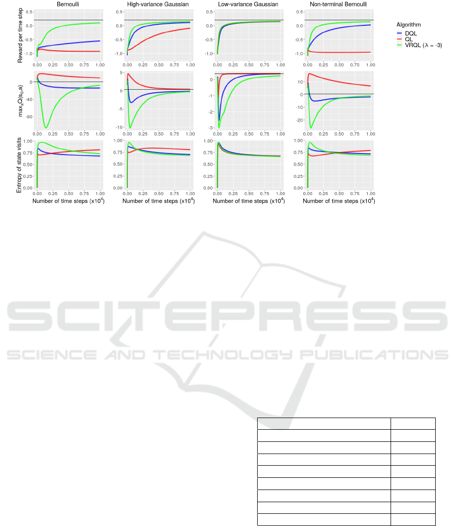
Figure 4: Results obtained from the grid world experiment. The reward per time step from the beginning of learning is shown

in the top row, the maximum action value of the starting state is shown in the middle row, and the normalized entropy of

the state visits is shown in the bottom row. Each column corresponds to a different reward function. The optimal values

are marked with black horizontal lines in the plots of the top and middle rows. The quantities were averaged over 10,000

simulations.

optimal action values of the non-goal states and ex-

plores the non-goal states for more steps when λ is

set to higher values.

4.2 Grid World with Function

Approximation

The environment used in our second experiment is a

similar grid world to the one used in our ﬁrst experi-

ment. The only difference is that the size of this world

is 10 × 10 instead of 3 × 3. The starting state is again

located at the bottom left corner and the goal state at

the top right corner.

In this experiment we used the function approx-

imation versions of the three algorithms with multi-

layer perceptrons as function approximators. At each

time step the current state was represented by a vector

with 200 binary elements that encoded the positions

of the agent and of the goal cell in the grid.

The reward functions used in this experiment are

identical to the ones used in the ﬁrst experiment.

Since an optimal policy ends the episode in 19 ac-

tions, the optimal expected reward per time step is

≈ −0.68. The discount factor was set to 0.99, and

therefore the maximum optimal action value of all

visited states per time step is ≈ −3.94 and the max-

imum optimal action value of the starting state is

≈ −12.38.

In table 1 we show the hyperparameters used in

this experiment, which were determined manually.

The action selection policy was ε-greedy, and ε was

linearly annealed from the initial exploration value to

the ﬁnal exploration value based on the exploration

decay steps value. For the multilayer perceptrons, we

used rectiﬁed linear units in the hidden layers, and

initialized all the weights with the Glorot uniform ini-

tializer (Glorot and Bengio, 2010). The total number

of steps in an experiment is 100,000 and each experi-

ment is repeated 5 times.

Table 1: Hyperparameters used in the grid world with func-

tion approximation experiment.

Hyperparameter Value

discount factor 0.99

initial exploration 0.5

ﬁnal exploration 0.01

exploration decay steps 150,000

learning rate 0.0025

number of hidden layers 1

number of hidden layer nodes 512

variation resistance parameter -0.5

Figure 5 shows the reward per time step from the

beginning of learning in the top row, the maximum

action value of all visited states per time step from

the beginning of learning in the middle row, and the

maximum action value of the starting state per time

step from the beginning of learning in the bottom row.

Each column corresponds to a different reward func-

tion, and the optimal value is marked with a black

ICAART 2021 - 13th International Conference on Agents and Artiﬁcial Intelligence

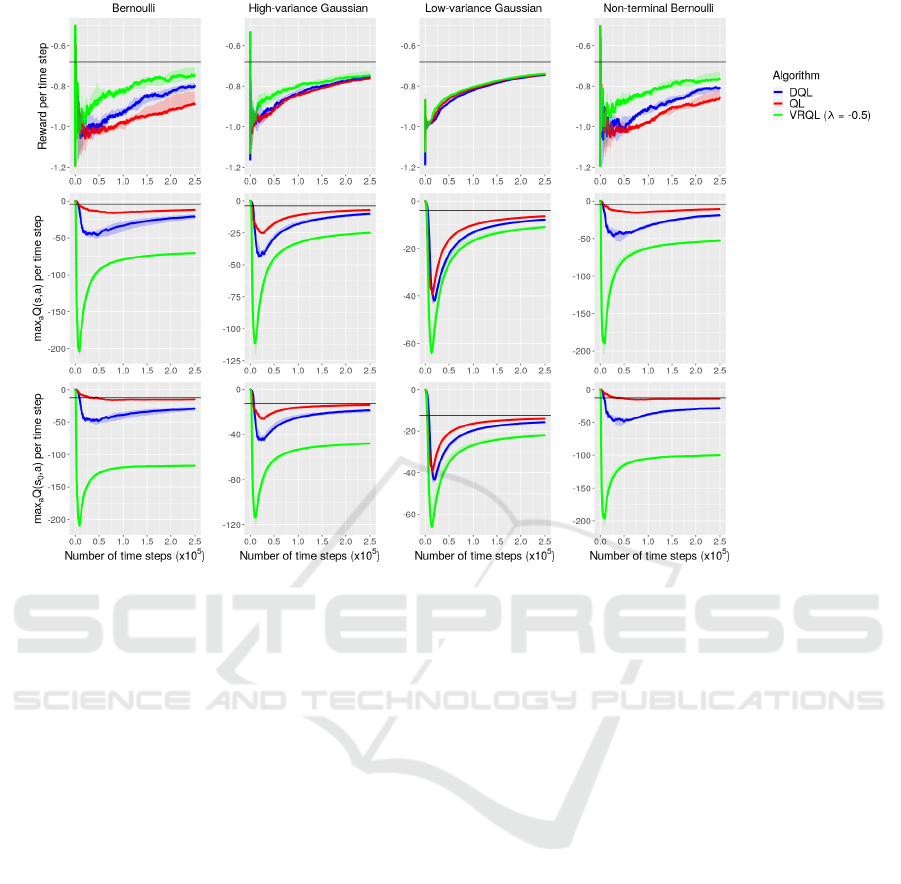
Figure 5: Results obtained from the grid world with function approximation experiment. The reward per time step from the

beginning of learning is shown in the top row, the maximum action value of all visited states per time step from the beginning

of learning is shown in the middle row, and the maximum action value of the starting state per time step from the beginning

of learning is shown in the bottom row. Each column corresponds to a different reward function. The optimal values are

marked with black horizontal lines. The quantities are median values over ﬁve simulations, and the shaded areas represent the

intervals between the mean of the two greatest values and the mean of the two least values.

horizontal line in each plot. The quantities are me-

dian values over ﬁve simulations with ﬁve different

random seeds, and the shaded areas represent the in-

tervals between the mean of the two greatest values

and the mean of the two least values.

Note that in the second experiment Variation-

resistant Q-learning and Double Q-learning were at

a disadvantage compared to Q-learning. In the case

of Variation-resistant Q-learning the reason is that the

algorithm had to allocate part of the capacity of its

multilayer perceptron to predict the absolute devia-

tions of the action-value estimates, whereas in the

case of Double Q-learning the reason is that the algo-

rithm updated the weight vector of only one of its two

multilayer perceptrons in each step. Nevertheless, the

results show that Variation-resistant Q-learning per-

formed better than Double Q-learning, and Double Q-

learning performed better than Q-learning. This hap-

pened for the same reasons as in the ﬁrst experiment.

Notice that Double Q-learning and Q-learning

performed better than in the ﬁrst experiment, although

the task of the second experiment was more difﬁcult

than the task of the ﬁrst experiment. The reason is that

the multilayer perceptrons generalized over the state

space and tried to learn the mean value of the update

targets for each action irrespective of the state.

Because of the behavior of the multilayer percep-

trons in this problem and also because the optimal

policy was not learned, all three algorithms underes-

timated the maximum optimal action values. Never-

theless, Variation-resistant Q-learning underestimated

the optimal values more than Double Q-learning, and

Double Q-learning underestimated the optimal val-

ues more than Q-learning. Underestimation was pos-

itively correlated with performance as expected.

Notice that the performance of all three algorithms

ﬂuctuated greatly in the beginning of learning. The

reasons are that the reward per time step was com-

puted with a limited amount of reward samples in the

beginning of learning and that the median values were

computed over only ﬁve simulations.

We also conducted experiments with the varia-

tion resistance parameter set to higher values and

Variation-resistant Q-learning behaved similarly to

the ﬁrst experiment as expected.

Variation-resistant Q-learning: Controlling and Utilizing Estimation Bias in Reinforcement Learning for Better Performance

4.3 Package Grid World

Figure 6 shows the 10 × 10 package grid world en-

vironment used in our third experiment. The agent’s

starting cell is the bottom left cell, the transitions are

deterministic, an attempt to move out of the world re-

sults in no movement, and there are ﬁve cells that con-

tain packages. Moreover, in addition to the four ac-

tions that cause transitions to neighboring cells, there

exists the action “collect”. This action results in no

movement, and if the agent’s cell contains an un-

collected package, the package is removed from the

world. The agent must collect all ﬁve packages in or-

der to end the episode.

Figure 6: A 10 × 10 package grid world. The agent’s start-

ing cell is the bottom left cell and there are ﬁve cells that

contain packages along the walls of the grid.

In this experiment we used the function approxima-

tion versions of the algorithms with multilayer per-

ceptrons as function approximators. At each time

step the current state was represented by a vector with

200 binary elements that encoded the positions of the

agent and of the uncollected package(s) in the grid.

The deterministic reward function provides a re-

ward of +100 for collecting all the packages, and a

reward of -1 per time step otherwise. Since the opti-

mal policy ends the episode in 32 actions, the optimal

expected reward per time step is ≈ 2.16. The discount

factor was set to 0.95, and therefore the maximum op-

timal action value of all visited states per time step is

≈ 40.47 and the maximum optimal action value of the

starting state is ≈ 4.47.

In table 2 we show the hyperparameters used in

this experiment, which we determined manually. The

action selection policy, the linear annealing procedure

of the exploration parameter, the activation functions

in the hidden layers of the multilayer perceptrons, and

the initialization of the weights of the multilayer per-

ceptrons were identical to the ones used in the second

experiment. Each run lasts for 1,000,000 steps.

In ﬁgure 7 we show the reward per time step from

Table 2: Hyperparameters used in the package grid world

experiment.

Hyperparameter Value

discount factor 0.95

initial exploration 1

ﬁnal exploration 0.05

exploration decay steps 750,000

learning rate 0.005

number of hidden layers 1

number of hidden layer nodes 256

variation resistance parameter +0.6

the beginning of learning in the left plot, the maxi-

mum action value of all visited states per time step

from the beginning of learning in the center plot, and

the maximum action value of the starting state per

time step from the beginning of learning in the right

plot. The optimal value is marked with a black hor-

izontal line in each plot. The quantities are median

values over ﬁve simulations with ﬁve different ran-

dom seeds, and the shaded areas represent the inter-

vals between the mean of the two greatest values and

the mean of the two least values.

Note that in the third experiment Variation-

resistant Q-learning and Double Q-learning were at

a disadvantage compared to Q-learning for the same

reasons as in the second experiment. This allowed

Q-learning to achieve superior performance in the

task of the third experiment. The reason is that in

this task it is relatively difﬁcult to discover the termi-

nal state, and therefore experiences with the terminal

state are relatively difﬁcult to sample. Q-learning uti-

lized those experiences better and followed good poli-

cies for more steps than the other two algorithms.

Double Q-learning performed worse than the

other two algorithms. The reason is that the task of

the third experiment does not favor underestimation.

As we mentioned above, in this task it is relatively

difﬁcult to sample experiences with the terminal state.

Moreover, the initial states are relatively far from the

terminal state, and therefore the optimal values of the

optimal and suboptimal actions in the initial states do

not differ a lot. Double Q-learning computed lower

estimates for the optimal values of the optimal ac-

tions than the other two algorithms in the beginning

of learning. This suggest that Double Q-learning ex-

plored suboptimal actions and followed bad policies

for more steps and that it needed more experiences

with the terminal state to determine the optimal ac-

tions than the other two algorithms.

We also conducted experiments with the varia-

tion resistance parameter set to lower values. As

λ decreases, the estimates of Variation-resistant Q-

learning for the maximum optimal action values grad-

ICAART 2021 - 13th International Conference on Agents and Artiﬁcial Intelligence

Figure 7: Results obtained from the package grid world experiment. The reward per time step from the beginning of learning

is shown in the left plot, the maximum action value of all visited states per time step from the beginning of learning is shown in

the center plot, and the maximum action value of the starting state per time step from the beginning of learning is shown in the

right plot. The optimal values are marked with black horizontal lines. The quantities are median values over ﬁve simulations

with ﬁve different random seeds, and the shaded areas represent the intervals between the mean of the two greatest values and

the mean of the two least values.

ually decrease and the performance of the algorithm

gradually becomes worse. This suggests that the algo-

rithm behaves similarly to Double Q-Learning when

λ is set to lower values as expected.

5 CONCLUSION

In this paper, we proposed Variation-resistant Q-

learning to control and utilize estimation bias for bet-

ter performance and showed empirically that the new

algorithm operates as expected. Although the argu-

ment that reinforcement learning algorithms can im-

prove their performance by controlling and utilizing

their estimation bias is unconventional, we think that

it is worth investigating further and hope that our

work will inspire further research on this topic.

Future Work. One future work direction would be

to provide a better theory for Variation-resistant Q-

learning, such as mathematically proving that the

variation resistance parameter can control the estima-

tion bias of the algorithm. Another future work di-

rection would be to conduct further experiments to

evaluate the algorithm. For example, the performance

of the algorithm could be tested on large-scale tasks

(e.g. in the video game domain) or tasks with non-

stationary environments. An additional future work

direction would be to improve the algorithm. Some

interesting improvements would be to determine the

variation resistance parameter automatically and to

provide functionality for the algorithm to arbitrarily

switch between overestimation and underestimation

during learning.

ACKNOWLEDGEMENTS

We would like to thank the Center for Information

Technology of the University of Groningen for their

support and for providing access to the Peregrine high

performance computing cluster.

REFERENCES

Anschel, O., Baram, N., and Shimkin, N. (2016).

Averaged-dqn: Variance reduction and stabilization

for deep reinforcement learning. arXiv preprint

arXiv:1611.01929.

Bellman, R. (1958). Dynamic programming and stochastic

control processes. Information and control, 1(3):228–

239.

D’Eramo, C., Restelli, M., and Nuara, A. (2016). Esti-

mating maximum expected value through gaussian ap-

proximation. In International Conference on Machine

Learning, pages 1032–1040.

Glorot, X. and Bengio, Y. (2010). Understanding the difﬁ-

culty of training deep feedforward neural networks.

In Proceedings of the thirteenth international con-

ference on artiﬁcial intelligence and statistics, pages

249–256.

Gordon, G. J. (1995). Stable function approximation in dy-

namic programming. In Machine Learning Proceed-

ings 1995, pages 261–268. Elsevier.

Lan, Q., Pan, Y., Fyshe, A., and White, M. (2020). Maxmin

q-learning: Controlling the estimation bias of q-

learning. arXiv preprint arXiv:2002.06487.

Lee, D., Defourny, B., and Powell, W. B. (2013). Bias-

corrected q-learning to control max-operator bias in

q-learning. In 2013 IEEE Symposium on Adaptive

Dynamic Programming and Reinforcement Learning

(ADPRL), pages 93–99. IEEE.

Singh, S., Jaakkola, T., Littman, M. L., and Szepesv

ari, C.

(2000). Convergence results for single-step on-policy

reinforcement-learning algorithms. Machine learning,

38(3):287–308.

Variation-resistant Q-learning: Controlling and Utilizing Estimation Bias in Reinforcement Learning for Better Performance

Sutton, R. S. and Barto, A. G. (2018). Reinforcement learn-

ing: An introduction. MIT press.

Thrun, S. and Schwartz, A. (1993). Issues in using function

approximation for reinforcement learning. In Pro-

ceedings of the 1993 Connectionist Models Summer

School Hillsdale, NJ. Lawrence Erlbaum.

Van Hasselt, H. (2010). Double q-learning. In Advances in

Neural Information Processing Systems, pages 2613–

2621.

Van Hasselt, H., Doron, Y., Strub, F., Hessel, M., Son-

nerat, N., and Modayil, J. (2018). Deep reinforce-

ment learning and the deadly triad. arXiv preprint

arXiv:1812.02648.

Van Hasselt, H., Guez, A., and Silver, D. (2016). Deep re-

inforcement learning with double q-learning. In Thir-

tieth AAAI conference on artiﬁcial intelligence.

Van Hasselt, H. P. (2011). Insights in reinforcement learn-

ing. PhD thesis, Utrecht University.

Watkins, C. J. and Dayan, P. (1992). Q-learning. Machine

learning, 8(3-4):279–292.

Watkins, C. J. C. H. (1989). Learning from delayed rewards.

PhD thesis, King’s College, Cambridge.

Zhang, Z., Pan, Z., and Kochenderfer, M. J. (2017).

Weighted double q-learning. In IJCAI, pages 3455–

3461.

APPENDIX

Deﬁnition 1. An ergodic Markov decision process is

a Markov decision process in which each state can

be reached from any other state in a ﬁnite number of

steps.

Lemma 1. Let (β

, ∆

, F

) be a stochastic process,

where β

, ∆

, F

: X 7→ R satisfy,

∆

t+1

) = (1 − β

))∆

) + β

)

where x

∈ X and t = 0, 1, 2, . . .. Let P

be a sequence

of increasing σ-ﬁelds such that β

and ∆

are P

measurable and β

, ∆

, and F

t−1

are P

-measurable,

with t ≥ 1. Assume that the following conditions are

satisﬁed:

1. The set X is ﬁnite (i.e.

< ∞).

2. β

) ∈ [0, 1],

∑

) = ∞,

∑

) < ∞ w.p.1,

and ∀x 6= x

: β

(x) = 0.

E{F

}

≤ κ

∆

+ c

, where κ ∈ [0, 1) and

−→ 0 w.p.1.

4. V{F

)| P

} ≤ C(1 + κ

∆

)

, where C is some

constant.

where V{·} denotes the variance and

denotes the

maximum norm. Then ∆

converges to zero with prob-

ability one.

Proof. See (Singh et al., 2000).

Theorem 1. In an ergodic Markov decision pro-

cess, the approximate action-value function Q as up-

dated by tabular Variation-resistant Q-learning in al-

gorithm 1 converges to the optimal action-value func-

tion q

∗

with probability one if an inﬁnite number of

experience tuples of the form (S

, A

, R

t+1

, S

t+1

) are

sampled by a learning policy for each state-action

pair and if the following conditions are satisﬁed:

1. The Markov decision process is ﬁnite (i.e. |S ×

A × R| < ∞).

2. γ ∈ [0, 1).

3. α

(s, a) ∈ [0, 1],

∑

(s, a) = ∞,

∑

(s, a) < ∞

w.p.1, and ∀s,a 6= S

, A

: α

(s, a) = 0.

Proof. We apply lemma 1 with X = S ×A, ∆

= Q

−

∗

, β

= α

, P

= {Q

, σ

, S

, A

, α

, R

, S

, . . . , S

, A

and

, A

) = R

t+1

+ γ

t+1

, A

∗

) − q

∗

, A

)

where A

∗

= argmax

t+1

, a

) and

t+1

, A

∗

) =

t+1

, A

∗

) + λσ

t+1

, A

∗

). The ﬁrst condition of

the lemma is satisﬁed because |S × A| < ∞. The sec-

ond condition of the lemma is satisﬁed by the third

condition of the theorem. The fourth condition of

the lemma is satisﬁed because

< ∞ =⇒ ∀t :

{

t+1

}

< ∞ =⇒ ∀t : V

{

, A

)| P

}

< ∞.

For the third condition of the lemma we have that,

, A

) = F

, A

) + γλσ

t+1

, A

∗

)

where F

, A

) is the value of F

, A

) in the

case of Q-learning. Since it is well known that ∀t :

E{F

}

≤ γ

∆

, it follows that,

E{F

}



E{F



}



+ γλ

{

≤ γ

∆

+ γλ

{

Therefore, it sufﬁces to show that c

γλ

{

→ 0 w.p.1.

Since ∀t, s, a : σ

(s, a) ∈ [0, ∞), it sufﬁces to show

that, lim

t→∞

, A

) = 0 ⇐⇒ ∀ε > 0 ∃t

: ∀t ≥

=⇒ σ

, A

) < ε. Assume that time step t is such

that the memory for each action value is full. We have

that,

, A

) =

∑

i=1



, A

) −

, A

)



where t

< t, ∀i = 1, 2, . . . , n. After the update at time

step t we have that,

t+1

, A

) =

∑

n+1

i=2



, A

) −

t+1

, A

)



where t

(n+1)

= t + 1. Because of the third con-

dition of the theorem, the differences between the

, A

) values approach zero as t → ∞. There-

fore, given ε > 0, ∃t

: ∀t ≥ t

=⇒ σ

, A

) < ε =⇒

lim

t→∞

, A

) = 0.

Since all the conditions of lemma 1 are satisﬁed,

it holds that, ∀s, a : Q

(s, a) → q

∗

(s, a) w.p.1.

ICAART 2021 - 13th International Conference on Agents and Artiﬁcial Intelligence