Combating Mode Collapse in GAN Training: An Empirical Analysis
using Hessian Eigenvalues
Ricard Durall
1,2,4
, Avraam Chatzimichailidis
1,3,4
, Peter Labus
1,4
and Janis Keuper
1,5
1
Fraunhofer ITWM, Germany
2
IWR, University of Heidelberg, Germany
3
Chair for Scientific Computing, TU Kaiserslautern, Germany
4
Fraunhofer Center Machine Learning, Germany
5
Institute for Machine Learning and Analytics, Offenburg University, Germany
Keywords:
Generative Adversarial Network, Second-order Optimization, Mode Collapse, Stability, Eigenvalues.
Abstract:
Generative adversarial networks (GANs) provide state-of-the-art results in image generation. However, despite
being so powerful, they still remain very challenging to train. This is in particular caused by their highly non-
convex optimization space leading to a number of instabilities. Among them, mode collapse stands out as
one of the most daunting ones. This undesirable event occurs when the model can only fit a few modes of
the data distribution, while ignoring the majority of them. In this work, we combat mode collapse using
second-order gradient information. To do so, we analyse the loss surface through its Hessian eigenvalues,
and show that mode collapse is related to the convergence towards sharp minima. In particular, we observe
how the eigenvalues of the G are directly correlated with the occurrence of mode collapse. Finally, motivated
by these findings, we design a new optimization algorithm called nudged-Adam (NuGAN) that uses spectral
information to overcome mode collapse, leading to empirically more stable convergence properties.
1 INTRODUCTION
Although Deep Neural Networks (DNNs) have ex-
hibited remarkable success in many applications, the
optimization process of DNNs remains a challenging
task. The main reason for that is the non-convexity
of the loss landscape of such networks. While most
of the research in the field has focused on single ob-
jective minimization, such as classification problems,
there are other models that require the joint mini-
mization of several objectives. Among these models,
Generative Adversarial Networks (GANs) (Goodfel-
low et al., 2014a) are particularly interesting, due to
their success of learning entire probability distribu-
tions. Since their first appearance, they have been
used to improve the performance of a wide range of
tasks in computer vision, including image-to-image
translation (Abdal et al., 2019; Karras et al., 2020),
image inpainting (Iizuka et al., 2017; Yu et al., 2019),
semantic segmentation (Xue et al., 2018; Durall et al.,
2019) and many more.
GANs are a class of generative models which con-
sist of a generator (G) and a discriminator (D) DNN
model. Within an adversarial game they are trained in
such a way that the G learns to produce new samples
distributed according to the desired data distribution.
Training can be formulated in terms of a minimax op-
timization of a value function V (G,D)
min
G
max
D
V (G, D).
(1)
While being very powerful and expressive, GANs are
known to be notoriously hard to train. This is because
their training is equivalent to the search of Nash equi-
libria in a high-dimensional, highly non-convex op-
timization space. The standard algorithm for solv-
ing this optimization problem is gradient descent-
ascent (GDA), where G and D perform alternating
update steps using first order gradient information
w.r.t. the loss function. In practise, GDA is often
combined with regularization, which has yield many
state-of-the-art results for generative models on var-
ious benchmark datasets. However, GDA is known
to suffer from undesirable convergence properties that
may lead to instabilities, divergence, catastrophic for-
getting and mode collapse. The latter term refers to
the scenario where only a few modes of the data dis-
tribution are generated and the model produces only a
limited variety of samples.
Many recent works have studied different ap-
proaches to tackle these issues. In reference (Rad-
ford et al., 2015), for instance, was one of the first
attempts to use convolutional neural networks in or-
Durall, R., Chatzimichailidis, A., Labus, P. and Keuper, J.
Combating Mode Collapse in GAN Training: An Empirical Analysis using Hessian Eigenvalues.
DOI: 10.5220/0010167902110218
In Proceedings of the 16th International Joint Conference on Computer Vision, Imaging and Computer Graphics Theory and Applications (VISIGRAPP 2021) - Volume 4: VISAPP, pages
211-218
ISBN: 978-989-758-488-6
Copyright
c
 2021 by SCITEPRESS – Science and Technology Publications, Lda. All r ights reserved
211

der to improve both training stability, as well as the
visual quality of the generated samples. Other works
achieved improvements through the use of new objec-
tive functions (Salimans et al., 2016; Arjovsky et al.,
2017), and additional regularization terms (Gulrajani
et al., 2017; Durall et al., 2020). There have also
been recent advances in the theoretical understanding
of GAN training. References (Nagarajan and Kolter,
2017; Mescheder et al., 2017), for examples, have in-
vestigated the convergence properties of GAN train-
ing using first-order information. There, it has been
shown that a local analysis of the eigenvalues of the
Jacobian of the loss function can provide guarantees
on local stability properties. Moreover, going beyond
first order gradient information, references (Berard
et al., 2019; Fiez et al., 2019) have used the top k-
eigenvalues of the Hessian of the loss to investigate
the convergence and dynamics of GANs.
In this paper, we conduct an empirical study to ob-
tain new insights concerning stability issues of GANs.
In particular, we investigate the general problem of
finding local Nash equilibria by examining the char-
acteristics of the Hessian eigenvalue spectrum and the
geometry of the loss surface. We thereby verify some
of the previous findings that were based on the top
k-eigenvalues alone. We hypothesize that mode col-
lapse might stand in close relationship with conver-
gence towards sharp minima, and we show empirical
results that support this claim. Finally, we introduce a
novel optimizer which uses second-order information
to combat mode collapse. We believe that our find-
ings can contribute to understand the origins of the
instabilities encountered in training GAN.
In summary our contributions are as follows
• We calculate the full Hessian eigenvalue spectrum
during GAN training, allowing us to link mode
collapse to anomalies of the eigenvalue spectrum.
• We identify similar patterns in the evolution of
the eigenvalue spectrum of G and D by inspect-
ing their top k-eigenvalues.
• We introduce a novel optimizer that uses second-
order information to mitigate mode collapse.
• We empirically demonstrate that D finds a local
minimum, while G remains in a saddle point.
2 RELATED WORK
While gradient-based optimization has been very suc-
cessful in Deep Learning, applying gradient-based al-
gorithms in game theory, i.e. finding Nash equilibria,
has often highlighted their limitations. An intense line
of research based on first- and second-order meth-
ods has studied the dynamics of gradient descent-
ascent by investigating the loss landscape of DNNs.
One of the initial first-order approaches (Goodfellow
et al., 2014b) studied the properties of the loss land-
scape along a linear path between two points in pa-
rameter space. In doing so, it was demonstrated that
DNNs tend to behave similarly to convex loss func-
tions along these paths. In later references (Draxler
et al., 2018) non-linear paths between two points were
investigated. There, it was shown that the loss surface
of DNNs contains paths that connect different min-
ima, having constant low loss along these paths.
In the context of second-order approaches, there
has also been notable progress (Sagun et al., 2016;
Alain et al., 2019). There, the Hessian w.r.t. the
loss function was used to reduce oscillations around
critical points in order to obtain faster convergence
to Nash equilibria. The main advantage of second-
order methods is the fact that the Hessian provides
curvature information of the loss landscape in all di-
rections of parameter space (and not only along the
path of steepest descent as with first-order methods).
However, this curvature information is local only and
very expensive to compute. In the context of GANs,
second-order methods have not been investigated in
depth. Recent works (Berard et al., 2019; Fiez et al.,
2019) have not calculated the full Hessian matrix but
resorted to approximations, such as computing the
top-k eigenvalues only. To the best of our knowledge,
we are the first to use the full Hessian eigenvalue spec-
trum to study the training behavior of GANs.
Another line of research tries to classify different
types of local critical points of the loss surface dur-
ing training w.r.t. their generalization behavior. In
(Hochreiter and Schmidhuber, 1997) it was originally
speculated that the width of an optimum is critically
related to its generalization properties. Later, (Keskar
et al., 2016) extended the conjectures by conducting
a set of experiments showing that SGD usually con-
verges to sharper local optima for larger batch sizes.
Following this principle, (Chaudhari et al., 2019) pro-
posed an SGD-based method that explicitly forces
optimization towards wide valleys. (Izmailov et al.,
2018) introduced a novel variant of SGD which av-
erages weights during training. In this way, solutions
in flatter regions of the loss landscape could be found
which led to better generalization. This, in turn, has
led to measurable improvements in applications such
as classification. However, (Dinh et al., 2017) argues
that the commonly used definitions of flatness are
problematic. By exploiting symmetries of the model,
they can change the amount of flatness of a minimum
without changing its generalization behavior.
VISAPP 2021 - 16th International Conference on Computer Vision Theory and Applications
212

3 PRELIMINARIES
3.1 Formulation of GANs
The goal of a generative model is to approximate a
real data distribution p
r
with a surrogate data distri-
bution p
f
. One way to achieve this is to minimize
the “distance” between those two distributions. The
generative model of a GAN, as originally introduced
by Goodfellow et al., does this by minimizing the
Jensen-Shannon Divergence between p
r
and p
f
, us-
ing the feedback of the D. From a game theoretical
point of view, this optimization problem may be seen
as a zero-sum game between two players, represented
by the discriminator model and the generator model,
respectively. During the training, the D tries to max-
imize the probability of correctly classifying a given
input as real or fake by updating its loss function
L
D
= E
x∼p
r
[log(D(x))] + E
z∼p
z
[log(1 −D(G(z))],
(2)
through stochastic gradient ascent. Here, x is a data
sample and z is drawn randomly.
The G, on the other hand, tries to minimize the
probability of D to classify its generated data cor-
rectly. This is done by updating its loss function
L
G
= E
z∼p
z
[log(1 −D(G(z))]
(3)
via stochastic gradient descent. As a result, the joint
optimization can be viewed as a minimax game be-
tween G, which learns how to generate new samples
distributed according to p
r
, and D, which learns to
discriminate between real and generated data. The
equilibrium of this game is reached when the G is
generating samples that look as if they were drawn
from the training data, while the D is left indecisive
whether its input is generated or real.
3.2 Training of GANs
As we explained above, the training of a GAN re-
quires the joint optimization of several objectives
making their convergence intrinsically different from
the case of a single objective function. The opti-
mal joint solution to a minimax game is called Nash-
equilibrium. In practice, since the objectives are
non-convex, using local gradient information, we can
only expect to find local optima, that is local Nash-
equilibria (LNE) (Adolphs et al., 2018). An LNE is
a point for which there exists a local neighborhood in
parameter space, where neither the G nor the D can
unilaterally decrease/increase their respective losses,
0.0 0.2 0.4 0.6 0.8 1.0
2.0
1.5
1.0
0.5
0.0
0.0 0.2 0.4 0.6 0.8 1.0
D(x)
0.0
0.2
0.4
0.6
0.8
1.0
D(G(z)
2.8
2.4
2.0
1.6
1.2
0.8
0.4
0.0
0.0 0.2 0.4 0.6 0.8 1.0
D(G(z)
2.0
1.5
1.0
0.5
0.0
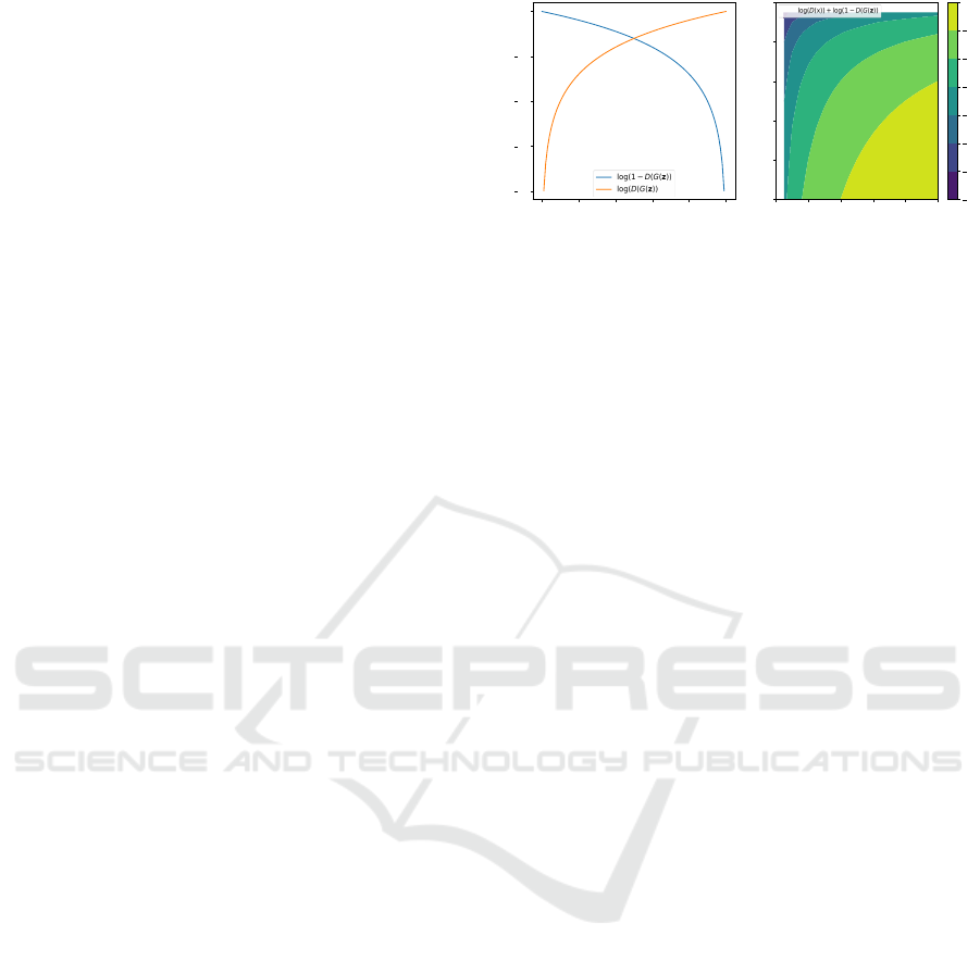
Figure 1: (Left) G losses, either minimization of log(1 −
D(G(z)) or maximization of log(D(G(z)). (Right) D loss,
maximization of log(D(x)) + log(1 −D(G(z)).
i.e. their gradients vanish while their second deriva-
tive matrix is positive/negative semi-definite:
||∇
θ
L
G
|| = ||∇
ϕ
L
D
|| = 0,
∇
2
θ
L
G
 0 and ∇
2
ϕ
L
D
 0
(4)
Here, θ and ϕ are the weights D and G, respectively.
3.3 Evaluation of GANs
GANs have experienced a dramatic improvement in
terms of image quality in recent years. Nowadays, it
is possible to generate artificial high resolution faces
indistinguishable from real images to humans (Karras
et al., 2020). However, their evaluation and compari-
son remain a daunting task, and so far, there is no con-
sensus as to which metric can best capture strengths
and limitations of models. Nevertheless, the Incep-
tion Score (IS), proposed by (Salimans et al., 2016),
is the most widely adopted metric. It evaluates images
generated from the model by determining a numerical
value that reasonably correlates with the quality and
diversity of output images.
4 METHOD
4.1 Non-Saturating GAN
In minimax GANs the G attempts to generate sam-
ples that minimize the probability of being detected
as fake by the D (c.f. Formula 3). However, in prac-
tice, it turns out to be advantages to use an alternative
cost function which instead ensures that the generated
samples have a high probability of being considered
real. This modified version of a GAN is called a non-
saturating GAN (NSGAN). When training a NSGAN
the G maximizes an alternative objective
E
z∼p
z
[log(D(G(z))].
(5)
The intuition why NSGANs perform better than
GANs is as follows. In case the model distribution
Combating Mode Collapse in GAN Training: An Empirical Analysis using Hessian Eigenvalues
213

is highly different from the data distribution, the NS-
GAN can bring the two distributions closer together
since the loss function generates a strong gradient. In
fact, the NSGAN will have a vanishing gradient only
when the D starts being indecisive whether its input is
from the data distribution or the G. This is accept-
able, however, since the samples will already have
reached the distribution of the real data by that time.
Figure 1 shows the loss function of the original and
non-saturating D and G, respectively.
4.2 Stochastic Lanczos Quadrature
Algorithm
During optimization the network tries to converge
into a local minimum of the loss landscape. Here we
differentiate between flat and sharp minima. Whether
a minimum is considered sharp or flat is determined
by the loss landscape around the converged point. If
the region has approximately the same error, the min-
imum is considered flat, otherwise we refer to the
minimum as sharp. Another method to determine the
sharpness of a minimum is by looking at the eigenval-
ues of the Hessian. These describe the local curvature
in every direction of the parameter space. This allows
us to see whether our network converges into sharp or
flat minima or whether it converges into a minimum
at all. Here, big eigenvalues correspond to a sharp
minimum in the corresponding eigendirection.
We observe that high eigenvalues in the G and D
lead to a worse IS score. Therefore we conclude that
mode collapse is linked to the network converging
into sharp minima. In order to confirm this, we look at
the full eigenvalue density spectrum during training.
Calculating the eigenvalues of the Hessian has a
complexity of O(N
3
), and storing the Hessian itself
in order to compute the eigenvalues scales with O(N
2
)
where N is the number of parameters in the network.
For neural networks that typically have millions of
parameters, calculating the eigenvalues of their Hes-
sian is infeasible. We can skip the problem of storing
the Hessian by only calculating the Hessian-vector
product for different vectors. In combination with
the Lanczos algorithm, this allows us to compute the
eigenvalues of the Hessian without having to calculate
and store the Hessian itself.
The stochastic Lanczos quadrature algorithm
(Lanczos, 1950) is a method for the approximation
of the eigenvalue density of very large matrices. The
eigenvalue density spectrum is given by
φ(t) =
1
N
N
∑
i=1
δ(t −λ
i
) (6)
where N is the number of parameters in the network,
λ
i
is the i-th eigenvalue of the Hessian and δ is the
Dirac delta function. In order to deal with the Dirac
delta function the eigenvalue density spectrum is ap-
proximated by a sum of Gaussian functions
φ
σ
(t) =
1
N
N
∑
i=1
f (λ
i
,t, σ
2
) (7)
where
f (λ
i
,t, σ
2
) =
1
σ
√
2π
exp(−
(t −λ
i
)
2
2σ
2
) (8)
We use the Lanczos algorithm with full reorthogonal-
ization in order to compute eigenvalues and eigenvec-
tors of the Hessian and to ensure orthogonality be-
tween the different eigenvectors. Since the Hessian is
symmetric we can diagonalize it and all eigenvalues
are real. The Lanczos algorithm is used together with
the Hessian vector product for a certain number of it-
erations. Afterwards it returns a tridiagonal matrix T .
This matrix is diagonalized as
T = ULU
T
(9)
where L is a diagonal matrix.
By setting ω
i
= U
2
1,i
and l
i
= L
ii
for i = 1, 2, ..., m,
the resulting eigenvalues and eigenvectors are used to
estimate the true eigenvalue density spectrum
ˆ
φ
(v
i
)
(t) =
m
∑
i=1
ω
i
f (l
i
,t, σ
2
) (10)
ˆ
φ
σ
(t) =
1
k
k
∑
i=1
ˆ
φ
(v
i
)
(t) (11)
For our experiments we use the toolbox from (Chatz-
imichailidis et al., 2019) which implements the
Stochastic Lanczos quadrature algorithm. This allows
to inspect and visualize the spectral information from
our models.
4.3 Nudged-Adam Optimizer
To prevent our neural network from reaching sharp
minima during optimization, we remove the gradi-
ent information in the direction of high eigenvalues.
This forces our network to ignore the sharpest min-
ima entirely and instead converge into wider ones.
Inspired by (Jastrzebski et al., 2018), we construct
an optimizer based on Adam (Kingma and Ba, 2014)
which ignores the gradient in the direction of the top-
k eigenvectors. In order to achieve this, we use the
existing Adam optimizer and remove the directions
of steepest descent from its gradient. This means that
given the top-k eigenvectors v
i
and the gradient g we
remove the eigenvector directions by
g
∗
= g −
k
∑
i=1
< g, v
i
> v
i
(12)
VISAPP 2021 - 16th International Conference on Computer Vision Theory and Applications
214

The resulting gradient g
∗
is now used by the regu-
lar Adam optimizer. Using this technique one can
modify a lot of different optimizers into their nudged
counterpart by using g
∗
instead of the true gradient.
The eigenvectors are computed by using the Lanc-
zos method together with the R-operator. This al-
lows fast computation of eigenvalues and eigenvec-
tors without having to store the full Hessian.
5 EXPERIMENTS
In this section, we present a set of experiments to
study the loss properties and the instability issues that
might occur when training a GAN. We first use the vi-
sualization toolbox to inspect the spectrum of GANs
during training, and to corroborate the problematic
search of an LNE. Then, we examine the k-top eigen-
values from the G and D, and their evolution through-
out the training. Finally, we introduce a novel op-
timizer, called nudged-Adam, to prevent mode col-
lapse and we test its performances on several datasets
to guarantee reliability across different scenarios.
5.1 Visualizing Loss Landscape
We start our experimental section with a loss land-
scape visualization that will serve us as a reference
point. We believe that building a solid background
will help to provide a better understanding of the non-
convergent nature of GANs, in particular concerning
the G. In order to do this, we track the spectral den-
sity throughout the entire optimization process. Our
main goal here is to gather evidences from the cur-
vature that visualizes the general problem of finding
LNEs. In order to carry out these experiments, we in-
dependently analyse the loss landscapes of the G and
of the D using their highest eigenvalue, respectively.
We employ the toolbox from (Chatzimichailidis
et al., 2019) to visualize the loss landscape and the
trajectory of our GAN during training. In this way,
we can gain some insights into the optimization pro-
cess that happens underneath. Note, that to obtain the
trajectory, we project all the points of training into the
2D plane of the last epoch. Figure 2 shows the land-
scape after training for 180 epochs on the NSGAN
setup. By inspecting the landscapes, we observe (1)
the D clearly finds a local minimum and descends to-
wards it, and (2) the G ends up in an unstable saddle
point, as suggested by the irregular landscapes sur-
rounding it. This findings agree with the aforemen-
tioned second-order literature (Berard et al., 2019).
Figure 2: Logarithmic loss landscapes with trajectory of
the same training run, visualized along eigenvectors cor-
responding to the two highest eigenvalues of NSGAN on
MNIST. (Left) G loss landscape. (Right) D loss landscape.
5.2 Eigenvalue Analysis
After having gained intuition of the training condi-
tions of GANs and their problem to find and remain
at an LNE, we now focus our attention on the issue
of mode collapse. In particular, we provide empirical
evidences of a plausible relationship between mode
collapse and the behaviour of the eigenvalues. To this
end, we evaluate the spectrum of our model through-
out the optimization process. More specifically, we
track the largest eigenvalues from the G and from the
D for each epoch, together with the IS.
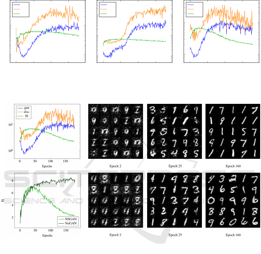
We start training and evaluating the original
non-saturating GAN architecture on the MNIST,
Kuzushiji, Fashion and EMNIST datasets (see Fig-
ure 3). This results in a number of patterns that are
present in all experiments. (1) The evolution of the
eigenvalues of the G and D behave visually very sim-
ilar. In particular, when D exhibits an increasing ten-
dency in its eigenvalues, the G does so as well. (2)
Apart from the G shape of the dynamics, it is impor-
tant to evaluate the local behaviour, i.e. the correlation
between the G and D. Thereby, we observe a strong
correlation in all our setups ranging from 0.72 to 0.90.
(3) Furthermore, there seems to exist a connection be-
tween the IS and the behaviour of the eigenvalues.
When the eigenvalues have a decreasing tendency, the
IS score tends to increase, while when the eigenvalues
increase, the IS scores deteriorates. Moreover, we see
how all our models start to suffer from mode collapse
after 25 epochs (approximately when the eigenvalues
tendency changes and starts to increase).
The empirical observations found in this analysis
lead to the conclusion that eigenvalues can give an
indication of the state of convergence of a GAN, as
pointed out in (Berard et al., 2019). Furthermore, we
found that the eigenvalue evolution is correlated with
the likely occurrence of a mode collapse event.
5.3 Combating Mode Collapse
In the last section we have seen that the growth of
Hessian eigenvalues during the training of a GAN cor-
Combating Mode Collapse in GAN Training: An Empirical Analysis using Hessian Eigenvalues
215

0
50
100
150
10
0
10
1
Epochs
gen
disc
IS
(a) Kuzushiji dataset. Correlation 0.80.
0
50
100
150
10
0
10
1
10
2
Epochs
gen
disc
IS
(b) Fashion dataset. Correlation 0.90.
0
50
100
150
10
0
10
1
Epochs
gen
disc
IS
(c) EMNIST dataset. Correlation 0.72.
Figure 3: Evolution of the top k-eigenvalues of the Hessian from generator (gen) and discriminator (disc), and the correspon-
dence IS over the whole training phase. The correlation score is measured between the G and the D.
Figure 4: (First row) Evolution of the top k-eigenvalues of the Hessian, the IS and random generated samples at different
epochs of NSGAN on MNIST. (Second row) Comparison of IS evolution of NSGAN and NuGAN, and random generated
samples at different epochs of NuGAN.
relates to the occurrence of mode collapse. In order to
remove this undesirable effect, we train our NSGAN
with a nudged-Adam optimizer (referred to as Nu-
GAN), which is inspired by (Jastrzebski et al., 2018).
Figure 4 shows the results together with some visual
samples generated at different training epochs. We
observe that NuGAN achieves a much more stable IS,
and this is also displayed on the generated samples.
While NSGAN suffers from mode collapse, NuGAN
does not (see samples on epoch 160). This shows
a clear relationship between the behaviour of the IS
score and the occurrence of mode collapse.
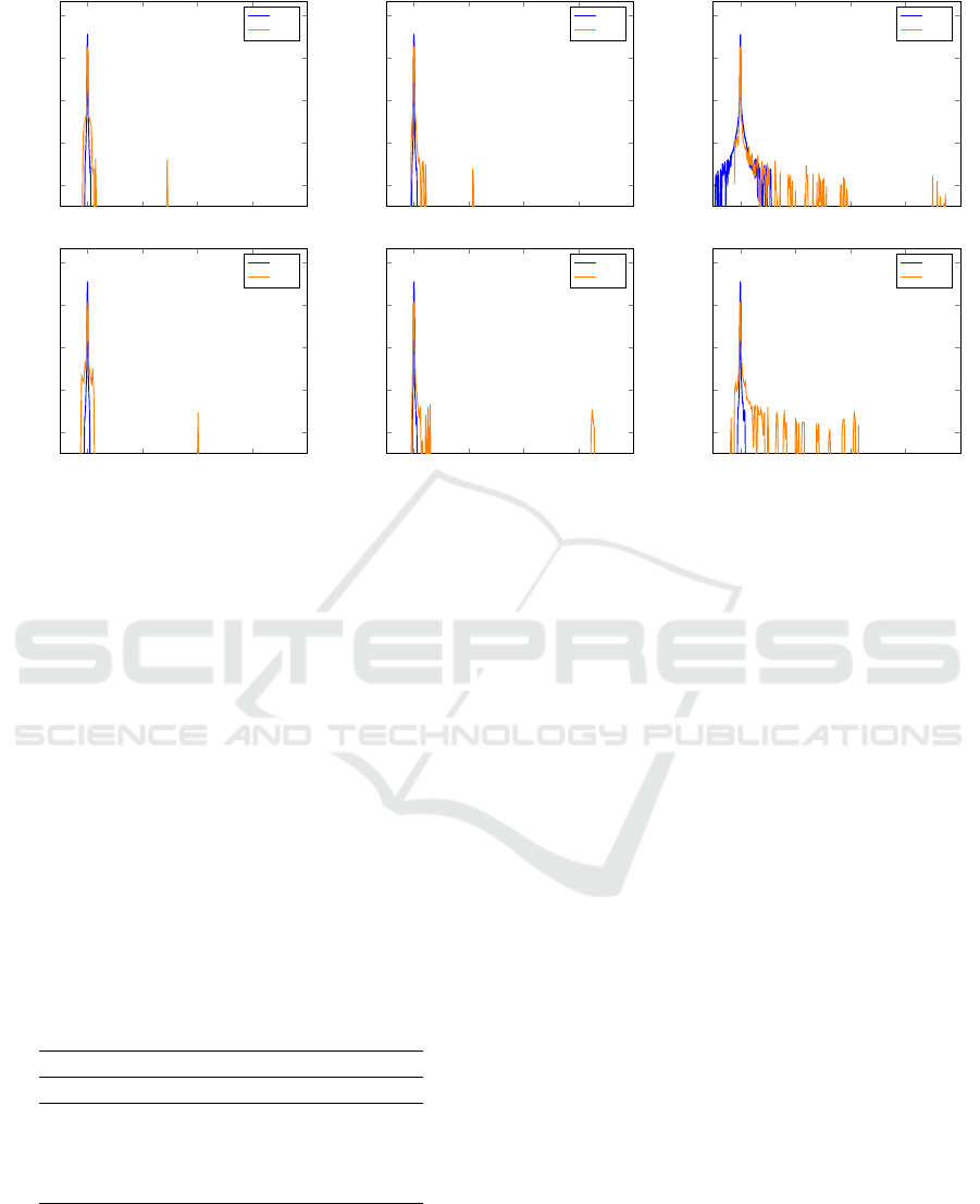
Figure 5 shows the full spectrum of the Hessian
at different stages of the training. A remarkable ob-
servation here is the present of negative eigenvalues
for the G for both optimizers. This indicates that the
critical point reached during training is not an LNE
(c.f. Formula 4). Rather, the G reaches only a saddle
point in all cases. On the other hand, the D seems to
converge to a sharp local minimum when using plain
GDA. In fact, it seems that the longer training lasts
the sharper the minimum gets. The D of our NuGAN
however, reaches a much flatter minimum, which can
be seen by the presents of much smaller eigenvalues
towards the end of training.
A second interesting observation is the connection
between the spectrum of the G and the mode collapse.
In particular, we observe the occurrence of mode col-
lapse when the spectrum spreads significantly (see
first row from Figure 5). On the other hand, the spec-
VISAPP 2021 - 16th International Conference on Computer Vision Theory and Applications
216

0 100 200 300 400
10
−7
10
−5
10
−3
10
−1
10
1
Eigenvalue
Hessian Eigenvalue Density
Epoch 2
gen
disc
0 100 200 300 400
10
−7
10
−5
10
−3
10
−1
10
1
Eigenvalue
Hessian Eigenvalue Density
Epoch 25
gen
disc
0 100 200 300 400
10
−7
10
−5
10
−3
10
−1
10
1
Eigenvalue
Hessian Eigenvalue Density
Epoch 160
gen
disc
0 100 200 300 400
10
−7
10
−5
10
−3
10
−1
10
1
Eigenvalue
Hessian Eigenvalue Density
gen
disc
0 100 200 300 400
10
−7
10
−5
10
−3
10
−1
10
1
Eigenvalue
Hessian Eigenvalue Density
gen
disc
0 100 200 300 400
10
−7
10
−5
10
−3
10
−1
10
1
Eigenvalue
Hessian Eigenvalue Density
gen
disc
Figure 5: Plots of the whole spectrum of the Hessian at different stage of the training on MNIST. (First row) Results on
NSGAN: we can identify an abnormal behaviour (mode collapse) in the generator at epoch 160. (Second row) Results on
NuGAN: the spectrum remains stable during the whole training. We can observe how the D for both cases finds local minima,
while the G remains all the time in a saddle point.
tral evolution of our NuGAN (see second row from
Figure 5) does not display any anomaly for the G, and
indeed, no mode collapse event occurrences. In Ta-
ble 1 we show more quantitative results supporting
the benefit of our nudged-Adam optimizer approach.
There we show the IS for both optimizers evaluated
of 4 different datasets. Notice that in all cases, our
method achieves a higher mean and maximum score
than the NSGAN baseline. These quantitative results
together with the visual inspection of the image qual-
ity suggest that our NuGAN algorithm has a direct
influence on the behavior of the eigenvalues and the
loss landscape of our adversarial model, resulting in
the avoidance of mode collapse.
Table 1: Mean and max IS from the different datasets and
methods (with and without mode collapse). Higher values
are better.
Methods NSGAN NuGAN
mean max mean max
MNIST 4.30 7.03 7.14 8.46
Kuzushiji 5.24 6.50 6.12 7.20
Fashion 5.74 6.82 6.35 7.20
EMNIST 3.77 7.02 8.53 7.67
Overall, we can summarize that the algorithm
does not converge to an LNE, while still achieving
good results w.r.t. the evaluation metric (IS). This
raises the question whether convergences to an LNE
is actually needed in order to achieve good generator
performance of a GAN.
6 CONCLUSIONS
In this work, we investigate instabilities that occur
during the training of GANs, focusing particularly on
the issue of mode collapse. To do this, we analyse
the loss surfaces of the G and D neural networks,
using second-order gradient information, with spe-
cial attention on the Hessian eigenvalues. Hereby,
we empirically show that there exists a correlation
between the stability of training and the eigenvalues
of the generator network. In particular, we observe
that large eigenvalues, which may be an indication
of the convergence towards a sharp minimum, corre-
late well with the occurrence of mode collapse. Mo-
tivated by this observation, we introduce a novel op-
timization algorithm that uses second-order informa-
tion to steer away from sharp optima, thereby prevent-
ing the occurrence of mode collapse. Our findings
suggest that the investigation of generalization prop-
erties of GANs, e.g. by analysing the flatness of the
optima found during training, is a promising approach
to progress towards more stable GAN training as well.
Combating Mode Collapse in GAN Training: An Empirical Analysis using Hessian Eigenvalues
217

REFERENCES
Abdal, R., Qin, Y., and Wonka, P. (2019). Image2stylegan:
How to embed images into the stylegan latent space?
In Proceedings of the IEEE international conference
on computer vision, pages 4432–4441.
Adolphs, L., Daneshmand, H., Lucchi, A., and Hof-
mann, T. (2018). Local saddle point optimization:
A curvature exploitation approach. arXiv preprint
arXiv:1805.05751.
Alain, G., Roux, N. L., and Manzagol, P.-A. (2019). Neg-
ative eigenvalues of the hessian in deep neural net-
works. arXiv preprint arXiv:1902.02366.
Arjovsky, M., Chintala, S., and Bottou, L. (2017). Wasser-
stein gan. arXiv preprint arXiv:1701.07875.
Berard, H., Gidel, G., Almahairi, A., Vincent, P., and
Lacoste-Julien, S. (2019). A closer look at the op-
timization landscapes of generative adversarial net-
works. arXiv preprint arXiv:1906.04848.
Chatzimichailidis, A., Keuper, J., Pfreundt, F.-J., and
Gauger, N. R. (2019). Gradvis: Visualization and sec-
ond order analysis of optimization surfaces during the
training of deep neural networks. In 2019 IEEE/ACM
Workshop on Machine Learning in High Performance
Computing Environments (MLHPC), pages 66–74.
IEEE.
Chaudhari, P., Choromanska, A., Soatto, S., LeCun, Y.,
Baldassi, C., Borgs, C., Chayes, J., Sagun, L., and
Zecchina, R. (2019). Entropy-sgd: Biasing gradient
descent into wide valleys. Journal of Statistical Me-
chanics: Theory and Experiment, 2019(12):124018.
Dinh, L., Pascanu, R., Bengio, S., and Bengio, Y. (2017).
Sharp minima can generalize for deep nets. CoRR,
abs/1703.04933.
Draxler, F., Veschgini, K., Salmhofer, M., and Hamprecht,
F. A. (2018). Essentially no barriers in neural network
energy landscape. arXiv preprint arXiv:1803.00885.
Durall, R., Keuper, M., and Keuper, J. (2020). Watch
your up-convolution: Cnn based generative deep neu-
ral networks are failing to reproduce spectral distribu-
tions. In Proceedings of the IEEE/CVF Conference
on Computer Vision and Pattern Recognition, pages
7890–7899.
Durall, R., Pfreundt, F.-J., K
¨
othe, U., and Keuper, J. (2019).
Object segmentation using pixel-wise adversarial loss.
In German Conference on Pattern Recognition, pages
303–316. Springer.
Fiez, T., Chasnov, B., and Ratliff, L. J. (2019). Convergence
of learning dynamics in stackelberg games. arXiv
preprint arXiv:1906.01217.
Goodfellow, I., Pouget-Abadie, J., Mirza, M., Xu, B.,
Warde-Farley, D., Ozair, S., Courville, A., and Ben-
gio, Y. (2014a). Generative adversarial nets. In
Advances in neural information processing systems,
pages 2672–2680.
Goodfellow, I. J., Vinyals, O., and Saxe, A. M. (2014b).
Qualitatively characterizing neural network optimiza-
tion problems. arXiv preprint arXiv:1412.6544.
Gulrajani, I., Ahmed, F., Arjovsky, M., Dumoulin, V., and
Courville, A. C. (2017). Improved training of wasser-
stein gans. In Advances in neural information pro-
cessing systems, pages 5767–5777.
Hochreiter, S. and Schmidhuber, J. (1997). Flat minima.
Neural Computation, 9(1):1–42.
Iizuka, S., Simo-Serra, E., and Ishikawa, H. (2017). Glob-
ally and locally consistent image completion. ACM
Transactions on Graphics (ToG), 36(4):107.
Izmailov, P., Podoprikhin, D., Garipov, T., Vetrov, D., and
Wilson, A. G. (2018). Averaging weights leads to
wider optima and better generalization. arXiv preprint
arXiv:1803.05407.
Jastrzebski, S., Kenton, Z., Ballas, N., Fischer, A., Bengio,
Y., and Storkey, A. (2018). On the relation between
the sharpest directions of dnn loss and the sgd step
length. arXiv preprint arXiv:1807.05031.
Karras, T., Laine, S., Aittala, M., Hellsten, J., Lehtinen,
J., and Aila, T. (2020). Analyzing and improving
the image quality of stylegan. In Proceedings of the
IEEE/CVF Conference on Computer Vision and Pat-
tern Recognition, pages 8110–8119.
Keskar, N. S., Mudigere, D., Nocedal, J., Smelyanskiy, M.,
and Tang, P. T. P. (2016). On large-batch training for
deep learning: Generalization gap and sharp minima.
arXiv preprint arXiv:1609.04836.
Kingma, D. P. and Ba, J. (2014). Adam: A
method for stochastic optimization. arXiv preprint
arXiv:1412.6980.
Lanczos, C. (1950). An iteration method for the solution of
the eigenvalue problem of linear differential and inte-
gral operators. United States Governm. Press Office
Los Angeles, CA.
Mescheder, L., Nowozin, S., and Geiger, A. (2017). The
numerics of gans. In Advances in Neural Information
Processing Systems, pages 1825–1835.
Nagarajan, V. and Kolter, J. Z. (2017). Gradient descent gan
optimization is locally stable. In Advances in neural
information processing systems, pages 5585–5595.
Radford, A., Metz, L., and Chintala, S. (2015). Unsu-
pervised representation learning with deep convolu-
tional generative adversarial networks. arXiv preprint
arXiv:1511.06434.
Sagun, L., Bottou, L., and LeCun, Y. (2016). Eigenvalues of
the hessian in deep learning: Singularity and beyond.
arXiv preprint arXiv:1611.07476.
Salimans, T., Goodfellow, I., Zaremba, W., Cheung, V.,
Radford, A., and Chen, X. (2016). Improved tech-
niques for training gans. In Advances in neural infor-
mation processing systems, pages 2234–2242.
Xue, Y., Xu, T., Zhang, H., Long, L. R., and Huang, X.
(2018). Segan: Adversarial network with multi-scale
l 1 loss for medical image segmentation. Neuroinfor-
matics, 16(3-4):383–392.
Yu, J., Lin, Z., Yang, J., Shen, X., Lu, X., and Huang, T. S.
(2019). Free-form image inpainting with gated con-
volution. In Proceedings of the IEEE International
Conference on Computer Vision, pages 4471–4480.
VISAPP 2021 - 16th International Conference on Computer Vision Theory and Applications
218