Fast Bridgeless Pyramid Segmentation for Organized Point Clouds

Martin Madaras

1,2 a

, Martin Stuchl

ık

1 b

and Mat

s Tal

ık

1,3 c

Skeletex Research, Slovakia

Faculty of Mathematics, Physics and Informatics, Comenius University Bratislava, Slovakia

Masaryk University Brno, Czech Republic

Keywords:

Point Cloud, Segmentation, Parallel, Pyramid, GPU, CUDA.

Abstract:

An intelligent automatic robotic system needs to understand the world as fast as possible. A common way to

capture the world is to use a depth camera. The depth camera produces an organized point cloud that later

needs to be processed to understand the scene. Usually, segmentation is one of the ﬁrst preprocessing steps

for the data processing pipeline. Our proposed pyramid segmentation is a simple, fast and lightweight split-

and-merge method designed for depth cameras. The algorithm consists of two steps, edge detection and a

hierarchical method for bridgeless labeling of connected components. The pyramid segmentation generates

the seeds hierarchically, in a top-down manner, from the largest regions to the smallest ones. The neighboring

areas around the seeds are ﬁlled in a parallel manner, by rendering axis-aligned line primitives, which makes

the performance of the method fast. The hierarchical approach of labeling enables to connect neighboring

segments without unnecessary bridges in a parallel way that can be efﬁciently implemented using CUDA.

1 INTRODUCTION

The world is moving towards automation. Robots are

picking parts from trays to assemble larger compo-

nents, cars can park themselves and cruise on high-

ways and 3D printers are self-correcting printing mis-

takes. All these applications are based on machines

understanding the surrounding world. One of the

principles is to determine where and what kind of ob-

jects are positioned in the space around the machine.

This is traditionally done by a depth camera and sub-

sequent processing of the input point clouds. When

capturing a stream of organized point clouds from a

3D camera, we need to process the stream of data

as fast as possible. The captured point cloud is im-

mediately processed by an image processing pipeline,

where segmentation is one of the most important pro-

cessing steps. The segmented point cloud is used as

an input to following processing algorithms and thus

the segmentation is used for the input data reduction.

Because the scanning artifacts result in bridges in the

thresholded pseudo-curvature metrics, it is not possi-

ble to use methods based on thresholding the metrics

https://orcid.org/0000-0003-3917-4510

https://orcid.org/0000-0001-8556-8364

https://orcid.org/0000-0002-3865-4507

and ﬂood-ﬁlling directly. Furthermore, segmentation

methods based on hierarchical clustering cannot be

efﬁciently implemented in a parallel way. The follow-

ing algorithm in the processing pipeline is performed

only using the subset of the input point cloud that is

needed for the optimal performance of the algorithm.

Therefore, efﬁciency and low execution time of the

segmentation process is crucial in all these robotics

applications.

The main contribution of the paper is a novelty

hierarchical parallel ﬁlling method that was designed

for fast pyramid segmentation of organized point

clouds (or directly depth maps with computed nor-

mal approximations). The proposed two-step method

modiﬁes the region ﬁlling algorithms such as a water-

shed or connected component labeling, into a fast and

robust method that ﬁlls the regions bridgelessly. The

ﬁlling is bridgeless even if the segmentation metrics

contains bridges between the regions after the thresh-

olding (bridges can be seen in Figure 1 and Section

3.3). The proposed method is directly applied on a

pseudo-curvature metrics computed from a set of in-

put organized point clouds captured by a 3D scanner.

The segmentation results are evaluated qualitatively

and the processing times are quantitatively compared

with other state of the art ﬁlling methods, bench-

marked on different CUDA compatible hardware.

Madaras, M., Stuchlík, M. and Tal

cík, M.

Fast Bridgeless Pyramid Segmentation for Organized Point Clouds.

DOI: 10.5220/0010163802050210

In Proceedings of the 16th International Joint Conference on Computer Vision, Imaging and Computer Graphics Theory and Applications (VISIGRAPP 2021) - Volume 4: VISAPP, pages

205-210

ISBN: 978-989-758-488-6

205

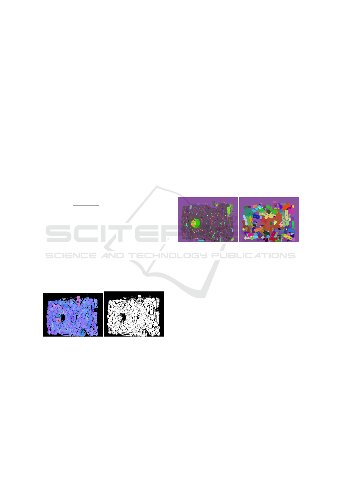
Figure 1: An input organized point cloud with estimated normals (left) is segmented into a set of regions where the region

boundaries are created either by high curvature or high depth differences, from which a segmentation metrics is calculated. The

pyramid segmentation starts by thresholding the metrics on different levels and constructing the label seeds in a hierarchical

way (middle). The seeds start to spawn from the largest areas on the highest level of the pyramid and they ﬁll the regions

by adding smaller seeds on lower levels. The hierarchical spawning of the seeds enables to eliminate the unwanted bridges

between the individual components. The ﬁnal bridgeless segmentation is shown on the right side, where the problematic areas

in the segmentation and the bridges in the thresholded metrics are marked by blue circles.

2 RELATED WORK

Existing algorithms for the segmentation of images

and structured point clouds can be divided into two

main groups, graph-based algorithms, and two-step

labeling algorithms. The graph-based algorithms

use a graph structure (Golovinskiy and Funkhouser,

2009) to iteratively merge over-segmented (Ben-

Shabat et al., 2017) image from previous itera-

tion steps. The algorithms usually start with one-

pixel regions (Felzenszwalb and Huttenlocher, 2004).

Due to hierarchical order of the performed merg-

ing steps, the parallelization on GPU cannot be per-

formed effectively enough to process 3-megapixel

depth camera scans in real-time (Abramov et al.,

2010). Some methods are based on pre-generation of

super-pixels (Lin et al., 2017; Fulkerson and Soatto,

2012; Achanta et al., 2012), that can be merged

more effectively, however the segment boundaries

do not match real interface between the objects. In

(Cheng et al., 2016), the authors used a hierarchi-

cal feature selection to merge the initial super-pixel

over-segmentation, which might result in wrong seg-

mentation if the initial super-pixels are not precise.

Two-step labeling algorithms ﬁrst start with the edge

detection step. Subsequently, the regions between

edges are ﬁlled with labels using watershed method

or connected component labeling algorithm (CCL)

(Ma et al., 2008). Computation of both steps can

be effectively parallelized (Allegretti et al., 2018; Al-

legretti et al., 2020), however the unwanted bridges

in the metrics are still the problem (see an exam-

ple of the computed metrics in Figure 2, right). An

extensive search for an efﬁcient way to perform la-

bel distribution among neighbors in parallel has been

made in (Hawick et al., 2010). Later, more advanced

approaches focusing on optimized, hardware speci-

ﬁed CUDA implementation have been proposed by

(Stava and Benes, 2011) and (Nina Paravecino and

Kaeli, 2014). An extensive evaluation on GPU CCL

approaches and block-based methods can be found

in (Asad et al., 2019). All the mentioned CCL ap-

proaches, with both CPU and GPU implementations,

share the same property that is unsuitable for our

case. The labeling results contain bridges between

segments that cause an intensive under-segmentation

(see Figure 3).

3 PYRAMID SEGMENTATION

To perform an efﬁcient two-step labeling algorithm

resulting in segmentation of the organized point cloud

(or depth map), the input needs to be processed by

computing the metrics and ﬁlling the regions between

boundaries in a parallel way. The pyramid segmenta-

tion is based on hierarchical seed spawning that was

inspired by a mipmap creation. The boundaries of the

thresholded metrics contain bridges and therefore, to

avoid under-segmentation, we construct the seeds in a

hierarchical manner and use the hierarchical informa-

tion to avoid the regions to overﬂow into neighboring

parts. If two seeds with different labels meet within

the bridge, according to the hierarchy level of the cur-

rently generated seed we know the size of the bridge.

By using the information about the bridge size, the

decision about seed merging can be made. In our ap-

proach, an input for the metrics calculation is an or-

ganized point cloud with estimated per point normals.

The normals can be estimated either in camera-space

(see Figure 1) or in calibration marker-space (see Fig-

ure 2). The 8-neighborhood of a point is deﬁned ex-

plicitly by iterating the one-ring in the grid structure

VISAPP 2021 - 16th International Conference on Computer Vision Theory and Applications

206

of the organized point cloud. Using the input, the met-

rics for region boundaries estimation is calculated and

thresholded ﬁrst and the initial seed spawns are cre-

ated inside the regions. Next levels of the labels in the

hierarchy are added iteratively, and the ﬁnal labeling

is performed in an efﬁcient line ﬁlling way inspired

by (Hemmat et al., 2015).

3.1 Metrics Calculation

In order to ﬁnd the boundaries between individual

scanned objects, we need to distinguish the interface

between the objects based on derivatives of available

per-point attributes in the input data; in the case of

point clouds captured by 3D scanners these avail-

able attributes are local curvature and local depth

derivatives. The segmentation metrics calculation is

based on the thresholding of two terms, a pseudo-

curvature term, and a depth-difference term. The

ﬁrst term, the pseudo-curvature c

is calculated as the

normalized sum of dot products between the point

normal and all the normals in the 8-neighborhood

= arccos(

∑

j∈8neigh

·n

8.0

), where n

is the normal of

the point and n

is the normal of the neighbor in the

8-neighborhood of the point). The second term, the

depth-difference d

, is the difference of the maximal

and the minimal differences in depth of neighbour-

ing points in the 8-neighborhood around the given

point (d

= max

j∈8neigh

i j

− min

j∈8neigh

i j

, where

i j

is the absolute depth difference in millimeters be-

tween point with index i and point with index j). Fi-

nally, these two terms are thresholded by thresholds ct

and dt in order to produce the ﬁnal metrics (see Fig-

ure 2, right) that will be ﬁlled in the next step of the

algorithm (see Figure 1, right).

Figure 2: (Left) the input point cloud with normals and

(right) computed and thresholded metrics resulting in the

edges.

3.2 Pyramid Filling

The computed metrics is converted into a binary im-

age using different level thresholds in the ﬁrst step.

Next, a pyramid of mipmaps is constructed (depicted

in Figure 1, middle), where the lowest resolution cor-

responds to the highest pyramid level while the orig-

inal binary image deﬁnes the lowest pyramid level.

When constructing a pyramid level, the value for a

texel is equal to zero if any of the values of four corre-

sponding texels from higher resolution pyramid level

is equal to zero. Otherwise, texel is labeled with a

value deﬁned as ﬁllable. After the pyramid is con-

structed, the algorithm runs through the pyramid from

the lowest to the original resolution. For each pyra-

mid level, texels marked as ﬁllable are labeled using

a value from lower resolution or a new unique label,

if the corresponding texel in a higher pyramid level is

not labeled and adding new labels at the current level

is enabled.

After labels are initialized, an iterative ﬂood-ﬁll

algorithm is deployed to ensure that texels with higher

values (or some unlabeled ﬁllable texels) are relabeled

by their lower-valued neighbors. For shorter execu-

tion time, the ﬂood-ﬁll algorithm is run in rows and

columns, using 4-neighborhood. At the lowest pyra-

mid level, labels may ﬁll an area one texel behind zero

labeled texels, as long as the edge detection step pro-

duces edges at least two texels wide.

Figure 3: (Left) the computed metrics is ﬁlled using CCL

and (right) the computed metrics is ﬁlled using our hierar-

chical bridgeless algorithm (using Scan03 and default pa-

rameters ct = 0.25, dt = 10).

3.3 Handling Bridges

Creating the segment boundaries by thresholding the

metrics often produces various small discontinuities

at detected edges, which we call bridges in the con-

text of this paper. The bridges are deﬁned as artifacts

in the computed metrics creating possible ﬂood ﬁll

paths. In the optimal segmentation result without the

artifacts, these possible ﬂood ﬁll paths should be cut

into different regions. By using simple CCL, even

the smallest bridge creates a connection between two

neighboring segments, which can lead to an intensive

under segmentation (see Figure 3, left). In contrast to

the CCL, the pyramid ﬁlling has some additional in-

formation about labels. By knowing the pyramid level

the label was created in, we can decide which segment

is (at least partly) wide enough to be sampled by a

given pyramid level. This allows rough approxima-

tion of minimal cuts between neighboring segments,

using a very simple heuristic (the comparison can be

seen in Figure 3). If there are two labels created in

Fast Bridgeless Pyramid Segmentation for Organized Point Clouds

207

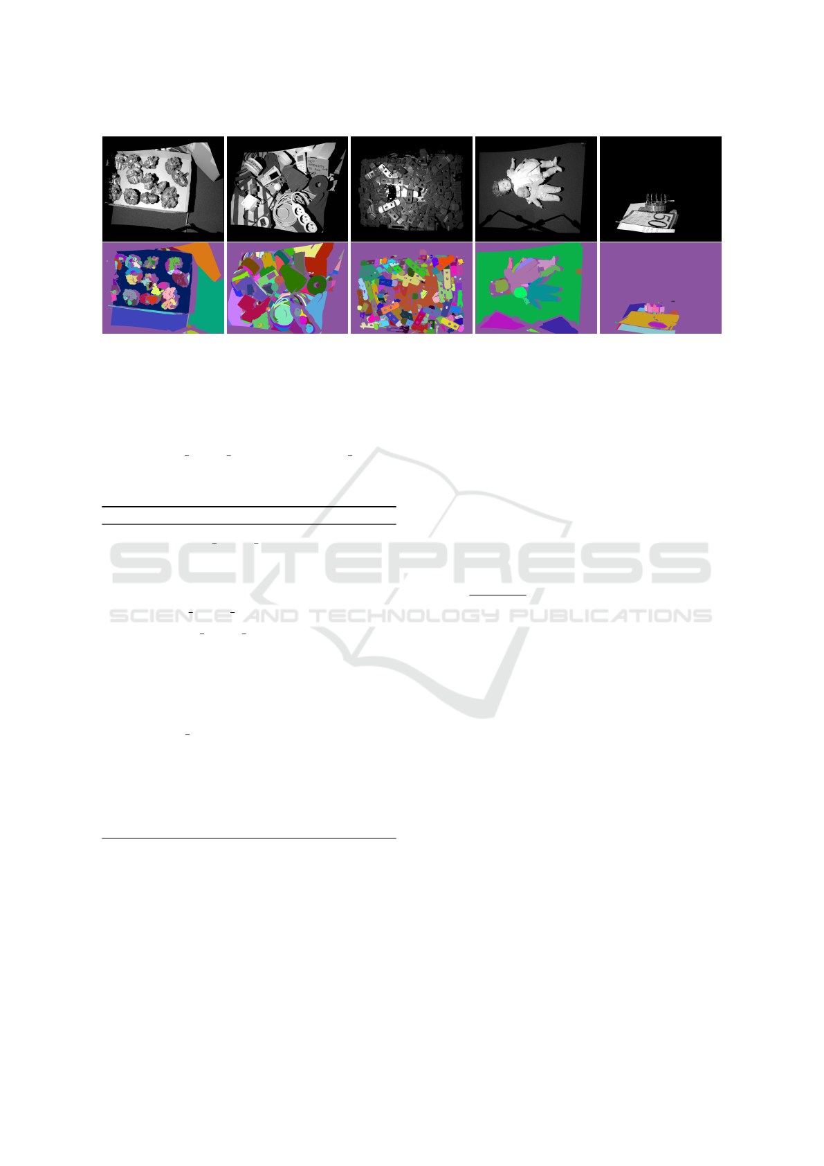
Figure 4: (Top) point clouds (Scan01 to Scan05) captured by Photoneo PhoXi 3D scanners that are used for the computation

time benchmark. (Bottom) results of pyramid segmentation using default parameters ct = 0.25, dt = 10.

one of the higher levels which were not joined in mul-

tiple previous levels a possible cut approximation is

detected. Let’s deﬁne a constructed pyramid P with

N levels indexed from 1 (highest level) to N (lowest

level). Let min bridge level and un joinable level be

pyramid level indices from 1 to N − 1. Then the algo-

rithm follows the following pseudocode:

Algorithm 1: Hierarchical Pyramid Segmentation.

1. for i in < 1,min bridge level >:

Initialize level[i] labels (addition of new labels is

enabled).

2. Run iterative ﬂood-ﬁll to join neighbouring labels

at level[min bridge level].

3. for i in < min bridge level + 1,N − 1 >:

Initialize level[i] labels (addition of new labels is

disabled).

4. Run ﬂood-ﬁll algorithm to join neighboring la-

bels at level[N − 1] (if both neighboring la-

bels were created in a level less or equal to

un joinable level, relabelling of higher value is

disabled).

5. Initialize level[N] labels (addition of new labels is

disabled).

6. Run one iteration of ﬂood-ﬁll (labeled texels are

ﬁlled only, relabeling of labeled ones is disabled).

4 CUDA IMPLEMENTATION AND

OPTIMIZATION

All passes of the algorithm can be directly translated

to CUDA code. However, two of the main passes,

metric calculation and ﬂood-ﬁll, will be slowed down

by inefﬁcient memory accesses.

In the metric calculation pass, each pixel is read

multiple times from the global memory. The duplicity

of loading from global memory is reduced by using

blocks of threads arranged in a 2D grid. A respective

2D tile of pixels including the border is loaded into

the shared memory in order to be processed. In the

ﬂood-ﬁll pass, naive use of one thread per row results

in non-coalesced accesses to the memory. To avoid

this, threads are grouped into blocks that ﬂood-ﬁll

their rows simultaneously. A block of threads always

loads a 2D tile of pixels in a coalesced manner into the

shared memory, processes them and then stores them

into global memory the same way. The process is re-

peated

width

tile/blocksize

times. The benchmarking showed

that for our GPUs the suitable number of threads per

block is 32 and the width of the tile is 32 as well,

therefore a tile loaded is 32x32 in size. The opti-

mization was performed for Nvidia Tegra TX1 and

TX2 processors, resulting in 32 block size. For clas-

sic modern desktop GPUs, a larger block size might

result in higher performance, however this optimiza-

tion oriented on standard GPUs was out of the scope

of our research.

5 COMPARISON AND

EVALUATION

A comparison of our proposed method to other seg-

mentation methods was performed on the same scans

and the same hardware (Scan01 and Nvidia GTX

1050 Ti was used). When compared to graph-based

methods, the CPU computation time of these meth-

ods is in seconds and it cannot be directly imple-

mented in parallel on GPU. For comparison with

other parallel GPU implementations of ﬁlling meth-

ods, the CCL (Hawick et al., 2010) CUDA imple-

mentation of the fastest test label-equivalence takes

VISAPP 2021 - 16th International Conference on Computer Vision Theory and Applications

208

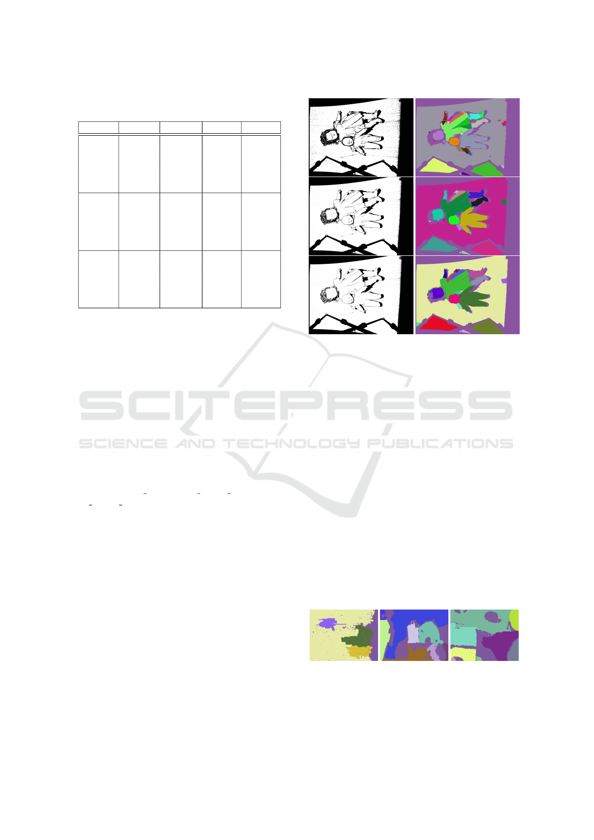
Table 1: Execution times in [ms] on Nvidia Tegra TX1, TX2

and GeForce GTX 1050 Ti GPU for organized point clouds.

Device Scan Metrics Segm. Total

TX1

Scan01 16.70 192.00 208.70

Scan02 14.60 224.00 238.60

Scan03 18.70 138.00 156.70

Scan04 13.13 159.00 172.13

Scan05 5.54 101.00 106.54

TX2

Scan01 12.10 69.25 81.35

Scan02 10.40 73.21 83.62

Scan03 13.50 56.59 70.09

Scan04 10.40 54.09 64.50

Scan05 3.96 50.94 54.90

1050Ti

Scan01 1.30 15.83 17.13

Scan02 1.25 19.72 20.97

Scan03 1.29 15.22 16.51

Scan04 1.29 16.54 17.83

Scan05 0.90 11.94 12.84

35.8ms in average, the quick-shift CUDA implemen-

tation (Fulkerson and Soatto, 2012) takes 341ms and

watershed GPU implementation (K

orbes et al., 2011)

takes 3018ms on Nvidia GTX 1050 Ti GPU for the

same input 3-megapixel point clouds. Our method is

faster (see Table 1) in comparison to other segmenta-

tion methods (50fps on GTX 1050 Ti), and it is able

to avoid small bridges between segments.

The visualization of the scans from Table 1 can

be seen in Figure 4. All the scans are with di-

mensions 2064 x 1544 captured by Photoneo PhoXi

structured light scanner (Photoneo, 2017). The pyra-

mid is constructed similarly to standard mipmaps

and depends only on the resolution of the input

scanned image. The experiments showed that op-

timal un joinable level is min bridge level − 2 and

min bridge level can be equal to N − 2 for most

datasets or to N − 3 for complicated datasets with

many bridges. The segmentation metrics based on the

depth and curvature is controlled by a pair of thresh-

old parameters ct, dt which different settings result

into a unique segmentation conﬁguration. By chang-

ing the threshold parameters ct, dt for thresholding

the pseudo-curvature term and the depth-difference

term, some edges might completely disappear from

the thresholded metrics as can be seen in Figure 5.

Thus, we were not able to evaluate the segmen-

tation results quantitatively. However, a qualitative

comparison of thresholded metrics ﬁlled using CCL

and our bridgeless approach can be seen in Fig-

ure 2. The quality metrics for segmentation eval-

uation depends on the use case of the processing

pipeline. In the robotics applications, where segmen-

tation is used, an over-segmentation is better than

under-segmentation. Thus, default values for the seg-

Figure 5: (Left) a computed metrics for the Scan04 where

the thresholding of the scan noise on different levels makes

a noticeable difference in the resulting edges. (Right) its

segmentation results mapped to scattered colors, with cur-

vature thresholds and distance thresholds (ct and dt) set to

0.15 and 1, 0.25 and 4, 0.35 and 10 (top to bottom).

mentation parameters ct and dt were empirically set

0.25 and 10, respectively. The best set of hyperpa-

rameters for our type of data was found experimen-

tally, they can be easily found for other 3D scanner

data with different resolution.

5.1 Limitations

The pyramid segmentation was designed to speed up

complex vision algorithms, where speed is prioritized

more than high-quality results. Rough pyramid ap-

proximations of minimal cuts may not be optimal and

can often be rectangularly jagged, while line based

ﬁlling can also introduce some small boundary ar-

tifacts (see Figure 6). The amount of artifacts usu-

ally correlates with data noise, which complicates the

edge detection and consequently the whole ﬁlling.

Figure 6: Our line ﬁlling approximation might result in

jagged boundary artifacts in locations, where the noise is

presented. The artifacts can be seen as lines that stick out

of the region boundaries, as depicted in the zoomed areas of

the scans.

Fast Bridgeless Pyramid Segmentation for Organized Point Clouds

209

We opted for a non-data-driven method for sev-

eral reasons. The main reason is missing data for the

training process. The data coming from the 3D scan-

ner have severe noise and we are not able to generate

synthetic ground truth labeled datasets for our struc-

tured light 3D scanners in an automatic way. Simulat-

ing a synthetic dataset for a structured light scanner

is non-trivial since it requires thorough capturing of

the scanning artifacts e.g. lens distortion, laser inter-

reﬂections, etc. As a result, while data-driven ap-

proaches can achieve very good results they are hard

to generalize to different scanning devices and their

speciﬁc reconstruction artifacts.

6 CONCLUSION

In this paper, a fast parallel method for image segmen-

tation has been proposed. The algorithm consists of

two steps, edge detection and hierarchical method for

labeling. Therefore, by using an alternative edge de-

tection algorithm, the pyramid segmentation may be

easily applicable to any other image data. The com-

ponent ﬁlling is a hierarchical approach that approxi-

mates the standard watershed and connected compo-

nent labeling algorithms. These algorithms are de-

signed for parallel implementation while hierarchical

seed spawning enables the removal of the unwanted

bridges between neighboring segments. The method

is suitable for real-time processing of the data cap-

tured by depth cameras and direct integration into var-

ious image processing, robotics, and computer vision

pipelines.

REFERENCES

Abramov, A., Kulvicius, T., W

org

otter, F., and Dellen, B.

(2010). Facing the multicore-challenge. chapter Real-

time Image Segmentation on a GPU, pages 131–142.

Springer-Verlag, Berlin, Heidelberg.

Achanta, R., Shaji, A., Smith, K., Lucchi, A., Fua, P., and

Susstrunk, S. (2012). Slic superpixels compared to

state-of-the-art superpixel methods. IEEE Trans. Pat-

tern Anal. Mach. Intell., 34(11):2274–2282.

Allegretti, S., Bolelli, F., Cancilla, M., and Grana, C.

(2018). Optimizing gpu-based connected components

labeling algorithms. In 2018 IEEE International Con-

ference on Image Processing, Applications and Sys-

tems (IPAS), pages 175–180.

Allegretti, S., Bolelli, F., and Grana, C. (2020). Optimized

block-based algorithms to label connected compo-

nents on gpus. IEEE Transactions on Parallel and

Distributed Systems, 31(2):423–438.

Asad, P., Marroquim, R., and e. L. Souza, A. L. (2019). On

gpu connected components and properties: A system-

atic evaluation of connected component labeling al-

gorithms and their extension for property extraction.

IEEE Transactions on Image Processing, 28(1):17–

31.

Ben-Shabat, Y., Avraham, T., Lindenbaum, M., and Fischer,

A. (2017). Graph based over-segmentation methods

for 3d point clouds. Computer Vision and Image Un-

derstanding, 174:12–23.

Cheng, M.-M., Liu, Y., Hou, Q., Bian, J., Torr, P., Hu, S.-

M., and Tu, Z. (2016). Hfs: Hierarchical feature se-

lection for efﬁcient image segmentation. In Leibe, B.,

Matas, J., Sebe, N., and Welling, M., editors, Com-

puter Vision – ECCV 2016, pages 867–882, Cham.

Springer International Publishing.

Felzenszwalb, P. F. and Huttenlocher, D. P. (2004). Efﬁcient

graph-based image segmentation. Int. J. Comput. Vi-

sion, 59(2):167–181.

Fulkerson, B. and Soatto, S. (2012). Really quick shift:

Image segmentation on a gpu. In Kutulakos, K. N.,

editor, Trends and Topics in Computer Vision, pages

350–358, Berlin, Heidelberg. Springer Berlin Heidel-

berg.

Golovinskiy, A. and Funkhouser, T. (2009). Min-cut based

segmentation of point clouds. In IEEE Workshop on

Search in 3D and Video (S3DV) at ICCV.

Hawick, K. A., Leist, A., and Playne, D. P. (2010). Par-

allel graph component labelling with gpus and cuda.

Parallel Comput., 36(12):655–678.

Hemmat, H. J., Pourtaherian, A., Bondarev, E., and de With,

P. H. N. (2015). Fast planar segmentation of depth im-

ages. In Image Processing: Algorithms and Systems.

orbes, A., Vitor, G. B., de Alencar Lotufo, R., and Fer-

reira, J. V. (2011). Advances on watershed process-

ing on GPU architecture. In Mathematical Morphol-

ogy and Its Applications to Image and Signal Pro-

cessing - 10th International Symposium, ISMM 2011,

Verbania-Intra, Italy, July 6-8, 2011, pages 260–271.

Lin, X., Casas, J. R., and Pard

as, M. (2017). 3d point cloud

segmentation using a fully connected conditional ran-

dom ﬁeld. 2017 25th European Signal Processing

Conference (EUSIPCO), pages 66–70.

Ma, N., Bailey, D. G., and Johnston, C. T. (2008).

Optimised single pass connected components anal-

ysis. 2008 International Conference on Field-

Programmable Technology, pages 185–192.

Nina Paravecino, F. and Kaeli, D. (2014). Accelerated

connected component labeling using cuda framework.

In Computer Vision and Graphics, pages 502–509,

Cham. Springer International P.

Photoneo (2017). Phoxi 3d scanner. https://www.photoneo.

com/products/phoxi-scan-m/.

Stava, O. and Benes, B. (2011). Connected component la-

beling in cuda. In Applications of GPU Computing

Series: GPU Computing Gems Emerald Edition.

VISAPP 2021 - 16th International Conference on Computer Vision Theory and Applications

210