
Attrition, Promotion, Transfer: Reporting Rates in Personnel
Operations Research
Etienne Vincent
1a
, Stephen Okazawa
2b
and Dragos Calitoiu
1c
1
Director General Military Personnel Research and Analysis, Department of National Defence, 101 Colonel By Drive,
Ottawa, Canada
2
Centre for Operational Research and Analysis, Department of National Defence, 101 Colonel By Drive, Ottawa, Canada
Keywords: Personnel Operations Research, Attrition Rate, Promotion Rate, Investment Performance Measurement.
Abstract: Rates of personnel flow, such as attrition, promotion and transfer, are widely reported, compared and modelled
in Personnel Operations Research (OR). However, different analysts commonly employ different formulas to
define these rates. This paper solidifies the foundation of Personnel OR by presenting a theoretically sound
formula for personnel flow rates that we will refer to as the general formula. The proposed formula is justified
by its properties, but also by analogy with the field of Investment Performance Reporting, where it is known
as the Time Weighted Rate of Return. The paper also derives approximation formulas for the rates of
personnel flow, and empirically compares them.
1 INTRODUCTION
Personnel Operations Research (OR) is the branch of
OR that supports operational decisions through
Human Resources (HR) data analysis and workforce
modelling. Practitioners of Personnel OR often
describe personnel flows using rates, such as attrition
rates, promotion rates and transfer rates. These rates
are reported, compared, and used within models, or as
the basis for forecasts. However, different
practitioners compute these rates in a variety of ways.
As pointed out by Noble (2011), all agree that the
attrition rate is important and that its definition is self-
evident, but then go on to give different definitions.
Common ways of defining attrition rates include
dividing the count of departing employees by the
period’s initial population, or alternatively by the
period’s average population (Bartholomew et al,
1991). Other denominators have also been employed.
For example, the Canadian Armed Forces have used
the sum of the initial population with half the number
of recruits (Okazawa, 2007). In general, different
attrition rate definitions attempt to account for the fact
that the size of the underlying population varies over
the period, but disagree on how to account for that
a
https://orcid.org/0000-0002-6877-2379
b
https://orcid.org/0000-0001-7287-6106
c
https://orcid.org/0000-0003-0173-9846
variation. Unfortunately, published work on this
subject is scarce. Most authors either report rates
without specifying a formula, or when they do present
a formula, do not present a theoretical justification.
We aim to solidify the foundation of Personnel
OR by introducing a definition for personnel flow
rates that we call the general formula. As such, we
generalize and improve on Okazawa (2007), the only
previous attempt to formally justify a personnel flow
rate formula of which we are aware. We will also
derive practical approximations of the general
formula, and empirically measures their accuracy.
2 PROPORTIONAL RATES
Attrition, promotion and transfer rates are
proportional rates. They represent the proportion of
a population that flows in a given direction, over a
given time period. For example, the attrition rate is
the proportion that leaves the organization entirely,
while a promotion rate tracks employees who move
to a higher pay grade. The treatment of proportional
rates by other disciplines can provide inspiration to
Personnel OR.
Vincent, E., Okazawa, S. and Calitoiu, D.
Attrition, Promotion, Transfer: Reporting Rates in Personnel Operations Research.
DOI: 10.5220/0010149001150122
In Proceedings of the 10th International Conference on Operations Research and Enterprise Systems (ICORES 2021), pages 115-122
ISBN: 978-989-758-485-5
Copyright
c
2021 by SCITEPRESS – Science and Technology Publications, Lda. All rights reserved
115
Proportional rates are omnipresent in
demographics. For example, mortality rates and
divorce rates are analogous to the attrition rates of
Personnel OR. However, demographic data often
come from multiple disparate sources, unlike
personnel data which is generally from a single HR
system. For example, divorces are promulgated by
courts and tracked by justice systems, whereas counts
of married couples come from censuses. This makes
it impossible to track day-to-day changes in the
married population, which would additionally require
reconciliation of immigration and mortality data from
yet other sources. Divorce rates, therefore, end up
being calculated as simple ratios between the numbers
of divorces and census population. Demographers also
rely on standardized rates, but this is outside our
current scope (Statistics Canada, 2017).
Proportional rates are also seen in the reporting of
subscription services churn rates, such as the
subscriber churn of wireless service providers. Such
reporting is widespread, and important to the fair
comparison of different carriers’ operational
prospects, but is not currently standardized. As an
example, AT&T reports the average over months, of
the number of subscribers who cancel service each
month divided by the number of subscribers at the
beginning of the respective months (AT&T, 2020).
Such a measure is reasonable, but not completely
satisfactory, as new subscribers are acquired during
the month, and some cancelling subscribers might not
have been there at the beginning of the month. This
area of proportional rate reporting is not yet mature
enough to inform the field of Personnel OR.
The discipline where proportional rates are most
mature is finance, where interest rates and rates of
return are crucial. In particular, Investment
Performance Measurement shares important
similarities with the reporting of rates in Personnel
OR. It is also highly standardized by regulatory
bodies, so as to allow a fair comparison of the returns
achieved by different investment firms. The
remainder of this section explores the rate formulas
used in Investment Performance Measurement.
2.1 Internal Rate of Return
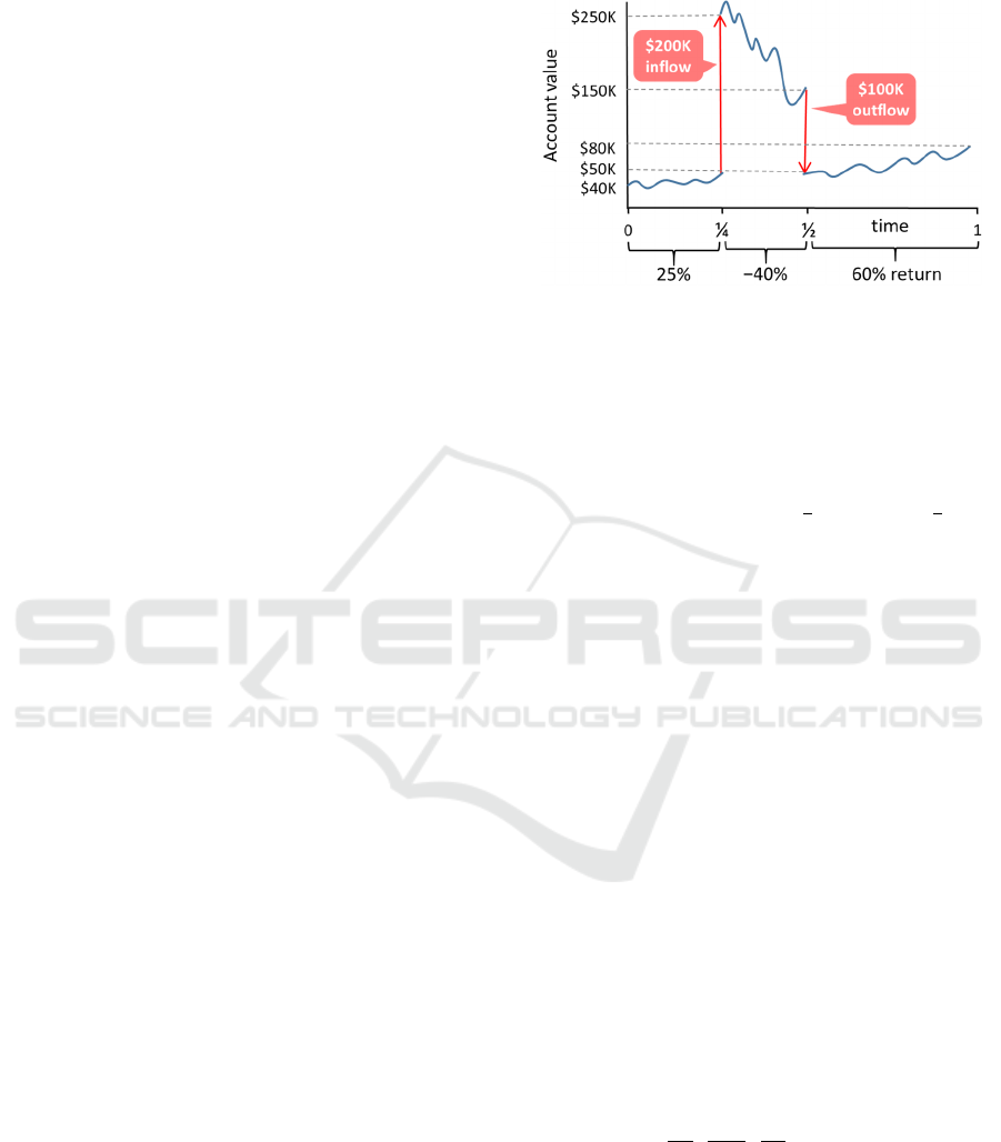
Consider Figure 1, which tracks the value of an
investment account over a year. Initially, the account
contains investments valued at $40K, which increase
in value to $50K within three months, representing a
25% increase. At that point, $200K is transferred into
the account. Over the next three months, the value of
the account drops to $150K – a 40% reduction, before
$100K is transferred out of the account. In the last six
months of the year, the value of the account grows by
60% from $50K to $80K.
Figure 1: Investment performance example.
The internal rate of return (IRR) is the effective
rate that achieves the account’s final value, when
applied to the initial value and the intervening cash
transfers. In our example, the IRR is of -42.0%, as
obtained by solving
8040
1
r
2001
r
1001
r
(1)
Regulators, such as the Canadian Securities
Administrators (CSA), require that the investment
performance of client accounts be reported using the
IRR or related metrics (CSA, 2017). However, the
IRR is not an appropriate performance measure for
investment fund managers. To see this, consider that
the IRR varies not only with the outcome of the fund
manager’s investment decisions, but also with the
amounts transferred in and out of the fund. Indeed,
with the example in Figure 1, the poor timing of the
external transfers is largely responsible for the loss,
and likely outside the control of the fund manager.
2.2 Time-weighted Rate of Return
The time-weighted rate of return (TWRR) is a
measure of investment performance that is invariant
with respect to external transfers. It is obtained by
compounding rates of return over the sub-periods
between each transfer. In our example, the TWRR is
of 20%, obtained as
50
40
∙
150
250
∙
80
50
1
(2)
This corresponds to the return that would have
resulted from a set investment, subject only to
changes in the value of the underlying assets (with no
external transfers). The TWRR is mandated by the
Chartered Financial Analyst (CFA) Institute’s Global
ICORES 2021 - 10th International Conference on Operations Research and Enterprise Systems
116

Investment Performance Standards for reporting
investment fund returns (CFA Institute, 2019).
3 RATES IN PERSONNEL OR
In Personnel OR, rates are often reported in order to
compare sub-populations (e.g. women versus men) or
to compare different periods (e.g. this year versus
last). For this, we need a measure that is invariant with
respect to other simultaneous flows (e.g. a measure
for promotions that is invariant to recruitment and
attrition flows). This is similar to the justification for
the TWRR. In the context of Personnel OR, we have
taken to referring to the TWRR as the general
formula for personnel flow rates. We first defined the
formula specifically for attrition rates, in a Canadian
Department of National Defence internal report
(Vincent et al, 2018).
The general formula can be used to measure
attrition, promotions, transfers, and all of their
variations. Of these, attrition (also called wastage by
some authors) is the most commonly reported. It is
the departure of employees for any reason
(resignation, retirement, dismissal, etc.). To simplify
the remainder of this paper, we often describe
concepts in terms of attrition rates, but remind the
reader that the discussion also applies to other
proportional rates of personnel flow.
3.1 The General Formula
Figure 2 shows the headcount, over a year, for a
workforce subject to attrition. For illustrative
purposes, attrition is atypically high in this example.
Figure 2: Example of attrition measurement.
The headcount starts at 6,250 and gradually
decreases. After the third month, 5,000 recruits show
up. Then, at the six month mark, 2,000 employees are
transferred out, perhaps the result of a spin-off – this
loss of personnel does not “count” as attrition. In the
end, 4,000 employees are left. In this example, the
general formula rate of attrition is of 55.2%, as
obtained by compounding the rates from the three
sub-periods that are free of other flows:
1
5,000
6,250
∙
7,000
10,000
∙
4,000
5,000
(3)
As with the TWRR, the general formula rate does
not vary with the timing of non-attrition flows.
Typically, HR data is captured at a daily resolution,
with inflows and outflows occurring between work
days. It is thus practical to express the general
formula as a compounding of daily rates:
1
a
(4)
where is the rate being measured, the number of
days in the period of interest, the headcount at
the end of the
th
day, and a the magnitude of the
relevant personnel flow on that day.
The general formula has two properties worth
highlighting. The first is that when a
is the only
flow affecting ,
a
1 for all ,
which leads to:
1
0
(5)
If at the same time, a denotes the magnitude of the
flow over the entire period, we also have
0a, such that Equation (5) can be re-cast as
a
0
(6)
The common definition of attrition rate as the
number of employees who depart divided by the
starting population is thus seen as a special case of the
general formula applicable when attrition is the only
flow.
The second property to highlight is that given sub-
period rates
, the general formula rate can simply
be obtained by compounding:
11
(7)
This multiplicative property directly follows from
Equation (4).
If the two desirable properties described by
Equations (5) and (7) are instead taken as a starting
point, we will notice that they are sufficient to derive
the general formula (Equation (4)). This is in fact how
Attrition, Promotion, Transfer: Reporting Rates in Personnel Operations Research
117
we first identified the general formula as our
preferred method for reporting attrition in (Vincent et
al, 2018). We only later drew parallels with
investment performance measurement.
3.2 Internal Rate of Personnel Flow
We now look at how the general formula must be
adapted in order to be applicable to the naïve forecasting
of future flows. This will lead us to the internal rate of
personnel flow – the analogue of the IRR.
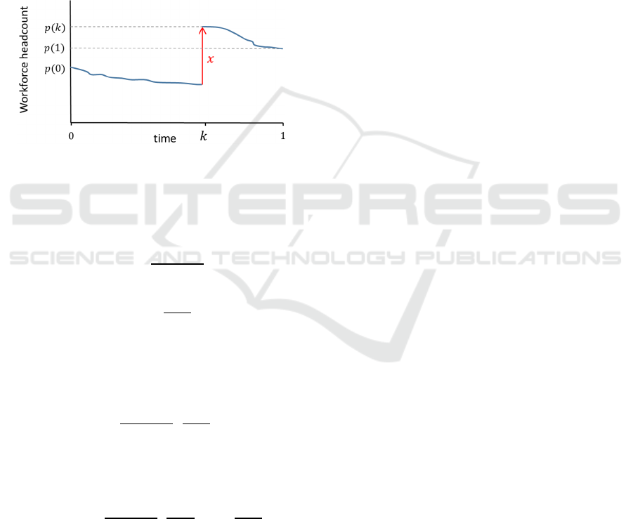
Figure 3 tracks a workforce undergoing a single
non-attrition flow of magnitude , perhaps the arrival
of a cohort of new hires, occurring at time .
Figure 3: Workforce with a single non-attrition flow.
Per Equation (5), the attrition rate over the sub-
periods without external flows are obtained from the
ratios of start/end headcounts as
1
,
0
(8)
1
,
1
(9)
with denoting the population immediately
before the non-attrition flow of magnitude . Per
Equation (7), attrition over the entire period
0,1
is
1
0
∙
1
(10)
Substituting Equation (10) into the following
easily verifiable identity
1
0
∙
0
∙
1
∙
1
(11)
we obtain
1
0
∙1∙1
,
(12)
Equation (12) separates the effect of attrition on
0
from its effect on , and may be generalized to
multiple non-attrition flows. Thus, given
0
and
knowledge of planned future non-attrition flows (i.e.
planned recruitment), Equation (12) can be used to
naïvely forecast attrition. However, doing this also
requires foreknowledge of
,
.
A reasonable assumption for
,
is that attrition
will advance at the same pace over
,1
, as over the
entire period:
1
,
≅1
(13)
Then, Equation (12) becomes
1
≅
0
∙1∙1
(14)
which, for an arbitrary number of external flows
occurring at times
, generalizes as
1
≅
0
∙1
∙1
(15)
We call Equation (15) the internal rate of personnel
flow. It can be understood as a model derived from the
general formula under an assumption of fixed paced
attrition throughout the period. This assumption is
unlikely to be strictly true in practice, but is reasonable
when nothing is known about the actual attrition
pattern, such as when forward-projecting a rate in order
to predict future attrition.
In Investment Performance Measurement, the
TWRR and IRR can give very different values, as was
seen with the example from Figure 1. In Personnel
OR, on the other hand, the rate from the general
formula and the internal rate of personnel flow are
typically much closer. This is because personnel
flows tend to occur at a steadier pace, and tend to be
small relative to the headcount.
4 RATE APPROXIMATIONS
The general formula defined by Equation (4) provides
a sound basis for measuring, reporting and comparing
personnel flows. However, applying it directly can
prove cumbersome in practice.
Say that we wanted to compare the attrition rates
of infantry and artillery captains. Applying the
general formula requires daily attrition counts, which
are easily extracted from HR System logs. It also
requires the daily population size for infantry and
artillery captains, which are typically harder to obtain.
That is because they must typically be derived from
transaction logs that track hiring, attrition,
promotions in and out of the rank of captain, and
ICORES 2021 - 10th International Conference on Operations Research and Enterprise Systems
118

occupation changes to and from infantry and artillery.
Coordinating all of these transactions can be delicate,
especially when some occur simultaneously, and
when the logs contain inconsistencies. Nevertheless,
code can be developed to solve the problem.
However, we might then want to compare the same
population segments, but only on a given military
base. Then, the code that determined daily
populations must be revised to consider posting
transactions to and from that base. If we are then
interested in further segmenting based on sex, age,
education or qualifications, the task of developing
code to derive accurate daily population sizes quickly
becomes overwhelming.
Approximation formulas that do not require daily
population sizes make easier the task of measuring
and comparing rates. This section derives such
formulas, while the next evaluates them empirically.
In general, we seek formulas for estimating
from
0
: the initial headcount,
1
: the headcount
at the end of the period (usually a year) and a: the
total attrition volume over the period. In practice,
when implementing such approximations, a is easily
extracted from the attrition transaction log, whereas
0 and 1 are taken from precomputed annual
workforce snapshots that list all employees along
with their relevant attributes (e.g. rank, occupation,
location, age, sex, etc.).
4.1 Half-intake Approximation
First, we set
1
0
a
(16)
as the net non-attrition flow in or out of the
workforce. For a given total attrition volume (a), the
value of given by Equation (4) varies with how a
and vary with respect to each other over the period
in question. To simplify Equation (4), we assume that
half of x occurs before all of a, itself followed by the
other half of , as shown in Figure 4.
Figure 4: Flows resulting in the half-intake approximation.
Then, attrition takes the headcount from
0
/2 down to
1
/2 without intervening non-
attrition flows. Using Equation (6), we get
≅
a
0
2
(17)
This formula is known as the Simple Dietz
method in the Investment Performance Measurement
literature, where it was originally derived in the
context of uncompounded returns (Dietz, 1966). In
Personnel OR, we have taken to calling it the half-
intake formula, as it is obtained by adding half of the
non-attrition flow (which often consists of new
recruits, or intake) to the denominator.
To obtain an expression based only on 0, 1
and a, we use Equation (16) and get
≅
2a
0
1
a
(18)
The half-intake formula was introduced to
Personnel OR by Okazawa (2007), based on a
derivation that was not tied to the general formula. It
has since become the most-often used attrition rate
measurement for the Canadian Armed Forces.
4.2 Uniform Taylor Approximation
Figure 4 yields a useful approximation formula, but is
a very artificial attrition pattern. A more realistic
assumption for many personnel flows is to distribute
them evenly across time. We have obtained a good
approximation when assuming uniformly distributed
net non-attrition flows, along with a constant pace of
attrition across the period, which amounts to assuming
that attrition behaves according to the internal rate of
personnel flow formula. When distributing
uniformly across time into Equation (15), we get
1 ≅ 0∙
1
1
(19)
In order to benefit from classical numerical
approximations for continuous functions, we map
Equation (19) to a continuous flow model:
1 ≅ 0∙
1
1
dt
(20)
which, through integration, becomes
1
≅
0
∙
1
∙
ln
1
(21)
Attrition, Promotion, Transfer: Reporting Rates in Personnel Operations Research
119

In order to avoid a numerical solution of Equation
(21) for , we use the Taylor series
ln
1
≅1
2
12
24
⋯
(22)
Then, to avoid having to numerically solve for ,
we only keep the quadratic terms. When substituted
into Equation (21), we obtain the quadratic polynomial
1
≅
0
∙
1
∙1
2
12
(23)
which solves for as
0
2
‐
0
2
3
01
6
(24)
when 0, and
0
1
/0 otherwise. We
refer to this as the uniform Taylor approximation
(denoted
).
Notice that if only the linear terms of Equation
(22) are kept, we get and alternative derivation of the
half-intake formula (Okazawa, 2007).
4.3 Mean Continuous Approximation
Like the uniform Taylor approximation, this one will
also be based on the internal rate of personnel flow.
First, we convert the periodically compounding rate
() to a continuously compounding rate (), as is
often done with rates of return in finance, by defining
ln1
(25)
When the conversion is applied to Equation (15),
the internal rate of personnel flow formula becomes
1≅0∙
∙
(26)
The attrition volume over
0,1
defined by
Equation (26) can be derived from Equations (16) as
a
0
1
≅0∙1
∙1
(27)
At the same time, the mean headcount over 0,1
defined by Equation (26) can be obtained by separating
the effect of attrition on the initial headcount 0
from its effect on each non-attrition flows
as
̅
≅0∙
∙
0∙1
∙1
(28)
Dividing Equation (27) by Equation (28), much
cancels out:
a
̅
≅
(29)
Because Equation (29) is a continuously
compounded rate obtained by dividing by the mean
headcount, we call it the mean continuous
approximation formula. Using Equation (25), we can
convert back to an annually compounding rate:
≅1
̅
⁄
(30)
Notice that no assumption was thus far made
about the pattern of non-attrition flows. Equation (30)
is essentially a reformulation of the internal rate
(Equation (15)). This is interesting because, Equation
(15) and the IRR are generally thought of as requiring
a numerical solution. The drawback of Equation (30)
is however that it relies on ̅, which is not readily
available.
We want an approximation based only on 0,
1 and a. The straightforward estimate of ̅ from
these values is
0
1
2
⁄
, which gives
≅
1exp
2a
0
1
(31)
It is interesting to note that Equation (29) is an
estimate of the attrition rate that is obtained by
dividing the attrition volume by the mean population
– a common definition of attrition used in Personnel
OR. However, as we have shown, this rate is correctly
understood as continuously compounding, and must
be converted to Equation (30), in order to represent
an annually compounding rate.
5 EMPIRICAL COMPARISON
The previous section derived three approximation
formulas. We now apply them to real-world data, in
order to find out how closely they approximate the
exact rates produced by the general formula.
We used Canadian Armed Forces Regular Force
data covering fiscal years 2009/10 to 2018/19. We
measured five different rates: overall attrition,
ICORES 2021 - 10th International Conference on Operations Research and Enterprise Systems
120

medical releases, Component Transfers (CT) from the
Regular Force to the Primary Reserve Force,
promotions, and Occupational Transfers (OT) –
transfers from one occupation to another, such as
from infantry to artillery. Each of the five rates was
calculated for 32 different workforce segments. The
segments were defined according to the following
attributes: age (older/younger than 40), Occupational
Authority (Army, Navy, Air Force and Assistant
Chief Military Personnel – which covers joint trades,
such as medical and logistics) and rank (junior and
senior segments for officers and for non-
commissioned members). Junior recruits, Generals
Officers, Chief Warrant Officers and Special Forces
were excluded. At the end of 2018/19, the largest of
the segments comprised 8,251 members, and the
smallest 183. In total, we thus conducted 1,600 tests
for each approximation formula: 5 rates 10 years
32 segments.
For each test, the exact general formula rate was
calculated using Equation (4), based on daily flow
volumes and headcounts. The rate approximations
were obtained using only annual figures: a, 0 and
1.
was calculated with Equation (18),
with Equation (24) and
with Equation (31).
5.1 Results
Table 1 shows the mean absolute differences between
the exact rates and corresponding approximations
over all conducted tests. It includes a row for each
type of rate investigated and the overall mean for the
1,600 tests of each approximation formula.
Table 1: Mean absolute difference between exact rates and
approximations.
Attrition 0.068931% 0.069231% 0.069488%
Medical 0.022225% 0.022386% 0.022508%
CT 0.008456% 0.008464% 0.008459%
Promotion 0.038723% 0.039441% 0.039422%
OT 0.027445% 0.027347% 0.027390%
Overall 0.032670% 0.032885% 0.032969%
All three formulas provide very close
approximations, especially given that personnel flow
rates are rarely reported with more than a tenth of a
percent precision. The best-performing
approximation formula in each row of Table 1 is
highlighted in green. We see that the half-intake
formula most often outperformed the others.
Table 2 looks at the worst cases among all tests,
rather than the mean. None of the three approximation
formulas clearly outperforms the others in Figure 2.
In all of the 1,600 tests conducted, none of the three
approximations were off by much more than 0.5%.
Table 2: Maximum absolute difference between exact rates
and approximations.
Attrition 0.504028% 0.506517% 0.502548%
Medical 0.159302% 0.162011% 0.163096%
CT 0.097457% 0.097575% 0.097451%
Promotion 0.330949% 0.354450% 0.355539%
OT 0.471317% 0.467894% 0.469390%
Overall 0.504028% 0.506517% 0.502548%
The differences between approximations and the
general formula were highest for those tests where the
population varied most, and when the personnel flow
being measured occurred near a population
extremum. For example, the worst differences from
Table 2 are for a segment where the headcount
dropped from 207 to 177, but not before peaking at
224 in July. Furthermore, most of the attrition that
year occurred in July near the peak.
Small errors in the measurement of a personnel
flow rate will rarely alter the conclusions of an
analysis. For example, if the goal of a study is to
highlight differences in the flows observed between
two segments (e.g. men and women), one would
likely only want to draw conclusions from flows that
differ by more than a percent. In our worst case, the
difference of 0.5% in a population of roughly 200
individuals amounts to a single person.
5.2 Using Monthly Snapshots
When a closer approximation is needed than can be
obtained from the methods investigated thus far, an
option is to use higher resolution data (e.g. monthly
headcounts and attrition volumes). If time is
measured in months rather than years, the previous
formulas can be reinterpreted as yielding monthly
(rather than annual) rates. To obtain an annual rate
from twelve monthly rates, the monthly rates need
only be compounded as follows:
1 1
(32)
Thus, Equation (32) can be combined with any
rate approximation formula applied to monthly data
Attrition, Promotion, Transfer: Reporting Rates in Personnel Operations Research
121

to yield better approximations. Table 3 presents the
absolute differences between exact rates and
approximations now derived from monthly data, over
the same 1,600 tests as before.
Table 3: Absolute difference between exact rates and rate
approximations derived from monthly data.
Mean
Difference
0.008974%
0.008957% 0.008959%
Maximum
Difference
0.241489%
0.240426% 0.241214%
In practice, the authors often use this approach.
We maintain database tables of monthly snapshots
that track relevant employee attributes, along with
transaction logs for attrition, promotions and
transfers. To measure a rate, we obtain monthly
headcounts from the snapshots, count the relevant
logged monthly transactions, estimate monthly rates,
and finally apply Equation (32).
Table 3 shows the uniform Taylor approximation
as marginally more accurate. However, it is harder to
communicate and less intuitive than the other two.
Before completing the present research, the authors
had used the half-intake formula for many years, and
Tables 1, 2 and 3 confirm that it produces accurate
estimates. We will thus continue to use the half-intake
formula for approximating reported rates.
Our results are based on Canadian Armed Forces
personnel data, which might not be representative of
other workforces. Personnel data is not generally
shared externally, for privacy reasons, but we would
like to invite others to replicate our tests within their
own organizations, so as to confirm of our results.
6 CONCLUSIONS
The goal of this paper was to lay a foundation for the
study of proportional rates in Personnel OR. We have
proposed the general formula for personnel flow rates
as that foundation, based on its properties. In addition,
we showed how the internal rate of personnel flow
can be derived from the general formula, and how it
offers a tool for the naïve forecasting of flows.
Finally, we justified the need for approximation
methods and provided options to obtain such
approximations. We showed empirically how our
proposed approximations are sufficiently accurate in
most cases, especially when computed from monthly
personnel data.
This paper addressed the need to appropriately
describe proportional rates in Personnel OR. We were
able to find inspiration from Investment Performance
Measurement, a field where the understanding of
proportional growth rates is fairly mature. However,
other fields still lack that depth of understanding. One
example is the reporting of churn rates for
subscription services. The specific requirements and
constraints of each field warrant their own
investigation, but the results of this paper can
hopefully inspire such investigation.
REFERENCES
AT&T, 2020. Q1 2020 AT&T Earnings – Financial and
Operational Trends, Author. Available at:
https://investors.att.com/financial-reports/quarterly-
earnings.
Bartholomew D. J., Forbes A. F. and McClean S. I., 1991.
Statistical Techniques for Manpower Planning, John
Wiley & Sons. Chichester.
CFA Institute, 2019. Global Investment Performance
Standards (GIPS
®
) For Firms – 2020, Author.
Charlottesville. Available at:
https://www.cfainstitute.org/en/ethics-
standards/codes/gips-standards.
CSA, 2017. Notice of Amendments to National Instrument
31-103, Author. Montreal. Available at:
https://www.osc.gov.on.ca/en/SecuritiesLaw_31-
103.htm.
Dietz, P., 1966. Pension Funds: Measuring Investment
Performance. Graduate School of Business, Columbia
University. New York.
Noble, S., 2011. Defining Churn Rate (No Really, This
Actually Requires an Entire Blog Post), Shopify
Engineering Blog. Available at:
https://shopify.engineering/defining-churn-rate-no-
really-this-actually-requires-an-entire-blog-post.
Okazawa, S., 2007. Measuring Attrition Rates and
Forecasting Attrition Volume (Technical Memorandum
DRDC CORA TM 2007-02), Defence Research and
Development Canada. Ottawa.
Statistics Canada, 2017. Age-standardized Rates, The
Daily, Author, Ottawa. Available at:
http://www.statcan.gc.ca/eng/dai/btd/asr.
Vincent, E., Calitoiu, D. and Ueno, R., 2018. Personnel
Attrition Rate Reporting (DGMPRA Scientific Report
DRDC-RDDC-2018-R238), Defence Research and
Development Canada. Ottawa.
ICORES 2021 - 10th International Conference on Operations Research and Enterprise Systems
122
