
Facial Exposure Quality Estimation for Aesthetic Evaluation
Mathias Gudiksen
1
, Sebastian Falk
1
, Lasse Nymark Hansen
1
, Frederik Brønnum Jensen
1
and Andreas Møgelmose
2
1
Department of Electronic Systems, Aalborg University, Denmark
2
Department of Architecture and Media Technology, Aalborg University, Denmark
Keywords:
Exposure Estimation, Aesthetic Evaluation, Handcrafted Features, Neural Network, Deep Learning,
Regression.
Abstract:
In recent years, computer vision systems have excelled in detection and classification problems. Many vision
tasks, however, are not easily reduced to such a problem. Often, more subjective measures must be taken into
account. Such problems have seen significantly less research. In this paper, we tackle the problem of aesthetic
evaluation of photographs, particularly with respect to exposure. We propose and compare three methods
for estimating the exposure value of a photograph using regression: SVM on handcrafted features, NN using
image histograms, and the VGG19 CNN. A dataset containing 844 images with different exposure values was
created. The methods were tested on both the full photographs and a cropped version of the dataset. Our
methods estimate the exposure value of our test set with an MAE of 0.496 using SVM, an MAE of 0.498
using NN, and an MAE of 0.566 using VGG19, on the cropped dataset. Without a face detector we achieve an
MAE of 0.702 for SVM, 0.766 using NN, and 1.560 for VGG19. The models based on handcrafted features
or histograms both outperform the CNN in the case of simpler scenes, with the histogram outperforming the
handcrafted features slightly. However, on more complicated scenes, the CNN shows promise. In most cases,
handcrafted features seem to be the better option, despite this, the use of CNNs cannot be ruled out entirely.
1 INTRODUCTION
Aesthetic assessment of photographs is a popular re-
search area in the field of computer vision, but the
problem is far from solved.
It can be used for a multitude of purposes. One
example is culling. During a photo session, photog-
raphers capture many more pictures than they need
(Tian et al., 2015). It is therefore important for a pho-
tographer to cull the photographs, such that only pho-
tographs of ”good” quality remain. The photographs
in Fig. 1 and Fig. 2 are examples of an aesthetically
pleasing photograph, and an aesthetically unpleasing
photograph, respectively. A photo may be culled be-
cause of duplicates, focus, exposure, facial expres-
sions, and poses among others. All of these measures
are difficult to quantify.
Automatic aesthetic evaluation may also be used
in search engines, where high quality photographs
should be presented at the top of the search results
(Tian et al., 2015)(Deng et al., 2017). Image quality
assessment is also often used in image editing soft-
ware (Lu et al., 2014) to provide the user with sug-
gested adjustments which improve the quality of the
photograph, for instance cropping and exposure.
This paper delimits the aesthetic evaluation prob-
lem to the perspective of solely looking at exposure
level of faces to be the problem to solve for now. If a
photo is not correctly exposed, it is discarded regard-
less of its other qualities, so exposure is a logical place
to start exploring automatic aesthetic evaluation. But
exposure is not just exposure. In almost all instances
where faces are present on pictures, the photographer
will want the faces to be correctly exposed, rather than
have a correct average exposure of the picture. Hence,
we investigate exposure estimation in a face-centric
perspective.
Figure 1: Photograph of
high aesthetic quality.
Figure 2: Photograph of low
aesthetic quality.
Gudiksen, M., Falk, S., Hansen, L., Jensen, F. and Møgelmose, A.
Facial Exposure Quality Estimation for Aesthetic Evaluation.
DOI: 10.5220/0010141102470255
In Proceedings of the 16th International Joint Conference on Computer Vision, Imaging and Computer Graphics Theory and Applications (VISIGRAPP 2021) - Volume 5: VISAPP, pages
247-255
ISBN: 978-989-758-488-6
Copyright
c
2021 by SCITEPRESS – Science and Technology Publications, Lda. All rights reserved
247

1.1 Related Work
Different types of metrics can be used to assess the
quality of photographs. These metrics can be grouped
into different levels:
• Technical metrics
• Subject metrics
• Composition metrics
• High-level metrics
Existing work does not necessarily take these lev-
els into account, but often looks at the task holisti-
cally - simply outputting an attractiveness score for
the input pictures, regardless of which metric level
they employ. Such a black-box approach may work,
but in order to understand the limitations of individual
systems, it is instructive to look at their level of met-
rics. After all, a system which solely evaluates, say,
colours will be unable to gauge the attractiveness of
the composition.
These levels are described in further detail below,
but before any of them can be evaluated, data must
be available. We point the reader toward some of the
different comprehensive datasets which do exist, such
as The Aesthetic Visual Analysis (AVA) (∼250.000
images) (Murray et al., 2012), Photo.Net (∼20.000
images)
1
, and the DPChallenge dataset (∼16.000 im-
ages)
2
. Each of them contain catalogues of images
which are rated by users from an aesthetic perspec-
tive (Deng et al., 2017).
Technical Metrics: describe the technical qualities
of the photo, such as exposure, sharpness, white bal-
ance, depth of field etc. (Marchesotti et al., 2011).
Research in methods for grading photographs based
on the technical metrics is well documented. Meth-
ods for computing various features and training a Sup-
port Vector Machine (SVM) to discriminate between
pleasing and displeasing photographs have been pro-
posed (Datta et al., 2006). Others have used Scale-
Invariant Feature Transform (SIFT) to extract key-
points and feature descriptors encoded in a Fisher
Vector to then classify using an SVM to determine
whether a photograph is pleasing or not, reaching an
accuracy of approximately 90% on the CUHK dataset
and 77 % on the Photo.net dataset.
Subject Metrics: are optimised for a specific cat-
egory of photographs, and hence the usable subject
metrics vary, depending on the subject. They are effi-
cient for a fixed task, known beforehand, but are not
generally applicable. If a photograph contains faces,
useful face-related subject metrics could be facial ex-
pressions, face symmetry, and face pose (Deng et al.,
1
http://photo.net
2
http://DPChallenge.com
2017). Research focusing on face-related regions by
using these three metrics, among others, to predict the
aesthetic quality have been made, achieving good re-
sults (Li et al., 2010).
Composition Metrics: relate to how the objects, and
especially the salient objects, are positioned relative
to each other, and relative to the scene. Simplicity
of the scene and balance among visual elements are
some of the indicators of good composition. These
composition metrics are also utilised to make salient
objects stand out more. Examples of composition
metrics are rule of thirds, low depth-of-field and op-
posing colours (Deng et al., 2017)(Obrador et al.,
2010). Researchers have explored the role of com-
position metrics in image aesthetic appeal classifica-
tion, focusing on simplicity and visual balance. They
achieved close to state-of-the-art image aesthetic-
based classification accuracy, only using composition
metrics (Obrador et al., 2010).
High-level Metrics: are hard to define, as they are
based on abstract concepts. High-level metrics can re-
late to either simplicity, realism or photographic tech-
nique, and designed high-level metrics such as spatial
distribution of edges, colour distribution and blur (Ke
et al., 2006). Some researchers have looked at the
content of images as high-level metrics, and present
the following content-based high-level metrics: pres-
ence of people, presence of animals and portrait de-
piction (Dhar et al., 2011).
Research in quality assessment of photographs
has, until recently, been focused on designing hand-
crafted features which can be used to distinguish be-
tween photographs of good or poor quality based on
different aesthetic measures, such as subject metrics
and high-level metrics (Guo et al., 2014)(Datta et al.,
2006)(Tong et al., )(Dhar et al., 2011). These hand-
crafted features were previously mostly based on a
combination of different metrics, such as the rule-
of-thirds, focus, exposure, colour combinations, etc.
These metrics were later largely replaced by generic
image descriptors such as Bag-Of-Visual-words and
Fisher Vectors (Marchesotti et al., 2011) in an attempt
to model photographic rules, using generic content
based features, which performs equal to, if not bet-
ter than the simple handcrafted features (Deng et al.,
2017). Lately, of course, research has been made
in employing Deep Convolutional Neural Networks
(CNN) in picking out the photographs of highest aes-
thetic quality (Tian et al., 2015). Deep learning meth-
ods may be able to generalise better across differ-
ent scenarios, whereas handcrafted methods are more
suited for specific tasks.
A unique approach (Kao et al., 2016) is look-
ing at dividing images into three different categories,
VISAPP 2021 - 16th International Conference on Computer Vision Theory and Applications
248

namely: ”scene” (covering landscapes, buildings
etc.), ”object” (covering portraits, animals etc.) and
”textures” (covering textures, images with sharp de-
tails etc.). A CNN is associated to each of these three
categories, thereby learning the aesthetic features for
the specific category and can then be used for mak-
ing an assessment of the photograph quality as either
a regression or a classification problem (Kao et al.,
2016).
Other researchers have extracted features from
a whole image as well as the face region specifi-
cally, and leveraged CNNs to train separate models
for the extracted feature sets, in order to evaluate the
influence of the background in aesthetic evaluation
(Bianco et al., 2018).
1.2 Our Approach
From the above, it is clear that previous studies have
shown that both handcrafted features and learned
deep features can be used in aesthetic quality assess-
ment. In this paper, we try to compare the meth-
ods by developing a system for exposure quality es-
timation of the face regions in photographs. This is
not a straight forward task, especially if the scene is
rather complex. In these scenarios the automatic ex-
posure setting in modern digital cameras tend to fail.
This approach allows for different types of stylistic
photographs, such as low and high key photographs,
where the background is either strongly over or under
exposed, but the faces are normally exposed. These
are edge cases which are poorly handled by existing
systems.
We define a set of handcrafted features and build a
regression on them. We then compare the results from
the handcrafted features with NN regression on image
intensity histograms as well as two CNNs trained to
give an output of an exposure estimate. The first CNN
is trained on images of faces extracted from the pho-
tographs and the second CNN is trained on the en-
tire photograph. This is done to determine whether
the network is able to automatically encode that our
region of interest when analysing exposure is faces,
such that a face detector can be avoided.
2 METHODS
2.1 Overview
An overview of the methodology in this paper is seen
in Fig. 3. Three different methods to estimate the ex-
posure of a photograph were developed: one using
handcrafted features, one using intensity histograms,
and one using a CNN. All three methods are tested
with both entire photographs, and with cropped out
faces as input.
Histogram
Handcrafted
Features
Input
Exposure
Estimate
Exposure
Estimate
CNN
Exposure
Estimate
Figure 3: Overview of the methodology in this paper.
2.2 Exposure Value
Exposure Value (EV) is used to determine which cam-
era setting combinations ensure the same exposure
of an image, given fixed illumination. Combina-
tions of the shutter speed and the aperture number
are found which yield the same exposure of an image.
By choosing a specific EV, we can adjust the shutter
speed to fit the needs for a given aperture. The EV
can be calculated as described in Eq. (1).
EV = log
2
N
2
t
(1)
where N is the f-number of the lens, and t is the
exposure time in seconds. Both values are encoded in
the EX metadata provided by the camera.
Different combinations of aperture and shutter
speed can result in the same EV, but are not guar-
anteed to result in the same image, since aperture
controls the depth of field, and shutter speed deter-
mines the amount of motion blur. For instance, an
EV = 13, which is appropriate for a bright day, may
be achived with f/1 and a shutter speed of 1/8000
s or a setting of f/4 with a shutter speed of 1/500
s. Shrinking the size of the aperture hole requires a
longer exposure time to compensate for the lower
amount of incoming light.
Lowering the EV increases the amount of light the
sensor will be exposed to, and vice versa. So to cap-
ture an image of a very bright scene, you simply ad-
just your EV to a suitably high positive value, e.g. EV
= 13. In most modern cameras this is done automati-
cally. An easy way to change the brightness of the re-
sulting picture is through EV compensation, which al-
lows the photographer to change the exposure ±3 EV,
with smaller increments in-between. If the photogra-
pher finds an image underexposed, they can simply do
Facial Exposure Quality Estimation for Aesthetic Evaluation
249
a compensation of +1 EV, which allows the camera to
change the settings to let in more light. Hence, a neg-
ative EV compensation value makes pictures darker
than the camera software deems appropriate, while a
positive value makes them lighter. In this paper, we
denote EV compensation as EV
c
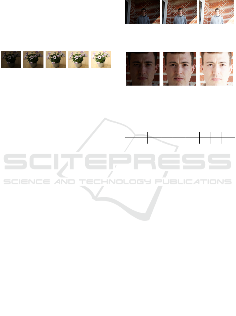
. To give a visual in-
tuition of how EV
c
influences a photograph, we refer
to the scale given in Fig. 4.
EV
c
= -2 EV
c
= -1 EV
c
= 0 EV
c
= +1 EV
c
= +2
Figure 4: Illustration of the exposure compensation brack-
eting method.
Images captured with a |EV
c
| ≥ 3 are either very dark,
bordering on black, or very bright. In a lot of cases
this means they are non recoverable. For overexposed
images, highlights are blown out, saturating the sen-
sor. In underexposed images, shadows are clipping,
meaning information is lost.
2.3 Dataset Acquisition
A dataset containing photographs with known EV
c
was needed to build our models. The datasets used by
(Marchesotti et al., 2011) are rated by users from an
online forum. In the Photo.Net dataset each image is
given a score ranging from 0 to 7, where 7 is the most
aesthetically pleasing photo. And in CUHK, images
have been given a binary aesthetic label followed by a
label regarding the scene, for instance, animals. None
of these are suited for the work in this paper.
The AVA dataset (Murray et al., 2012) contains
around 250.000 images. Of these, 50.000 images con-
tain metadata. However, not all images had a person
as subject and the exposure was not necessarily re-
lated to faces. As it was not possible to find a dataset
of images with ground truth EV
c
available, a dataset
was created. The images in the dataset have variance
in both background, lighting, aspect ratio, resolution,
size of faces, and have −3 ≤ EV
c
≤ 3. It features six
different people, both male and female, and the pho-
tographs are taken both indoors and outdoors. The
dataset contains a total of 844 images. Another ver-
sion of the dataset was compiled where all pictures
are cropped to show only the faces from the original
dataset. This was done using an off-the-shelf face de-
tector. An example of an underexposed, a normal ex-
posed and an overexposed image from the dataset can
be seen in Figs. 5 to 7, while the cropped faces can be
seen in Figs. 8 to 10.
Figure 5:
Underexposed
image from
dataset.
Figure 6:
Normal exposed
image from
dataset.
Figure 7:
Overexposed
image from
dataset.
Figure 8: Cropped,
underexposed.
Figure 9: Cropped,
normal exposed.
Figure 10:
Cropped,
overexposed.
The 844 images are distributed on the seven different
labels as seen in Table 1.
Table 1: Distribution of the data, according to label.
Label -3 -2 -1 0 1 2 3
Amount 144 87 116 208 64 89 136
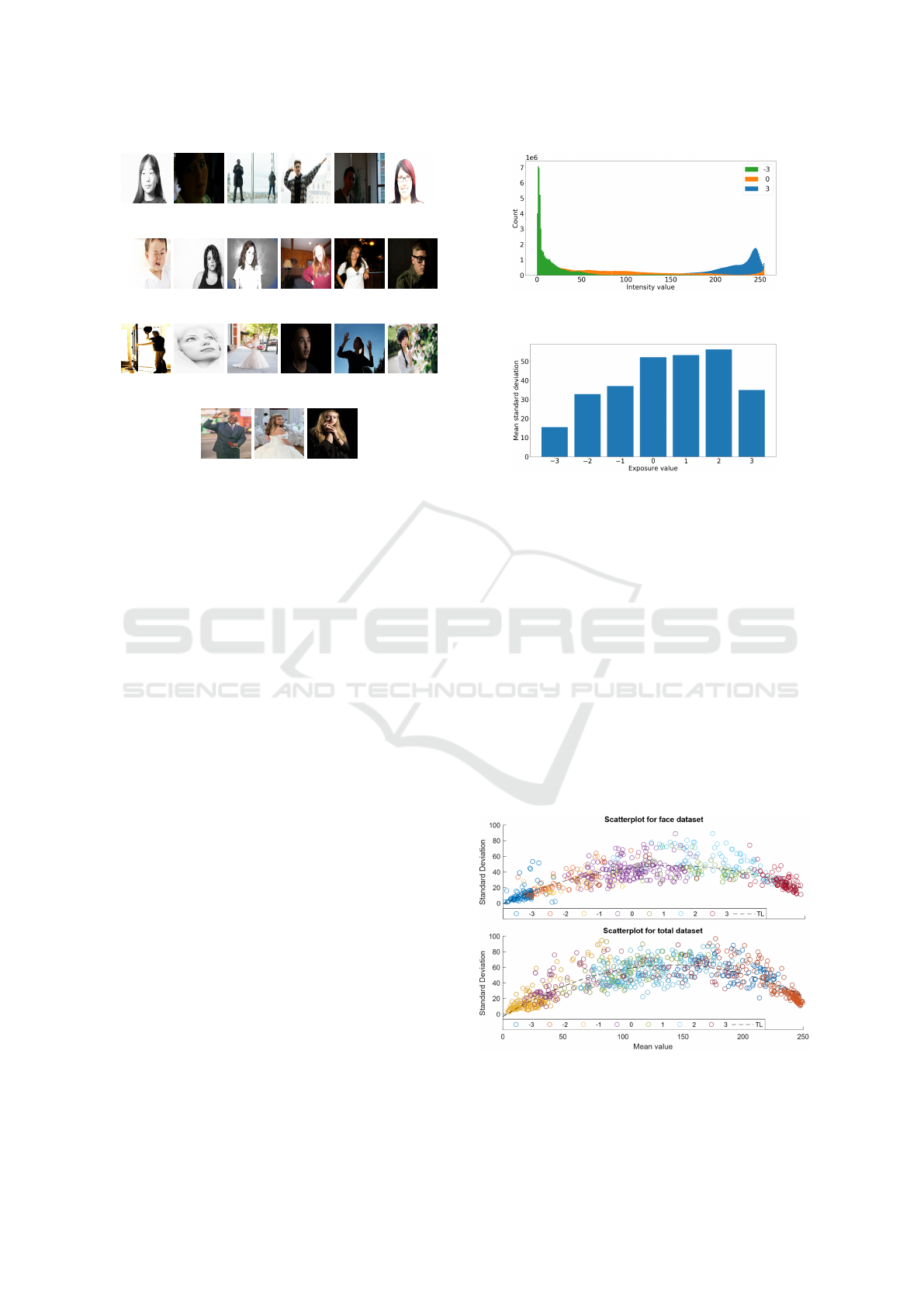
To test the methods developed in this paper, a sepa-
rate test set was compiled. This test set consists of
images similar to the ones found in the training data,
seeing as the images were acquired in much the same
fashion. This test set will be used as the base-line
for gauging the performance of the methods. To re-
ally push the methods to the limits, a second stress
test set was also compiled. This second test set was
compiled by finding relevant but stylistically differ-
ent images, spanning the edge cases which might oc-
cur in real operation. This set contains 21 images.
To prevent any overlap between the training data and
the stress test set, the stress test pictures were selected
among Creative Commons-licensed (Attribution 2.0
3
)
pictures from Flickr. We chose images for the second
test set which are supposed to stress the methods. For
example, in images 4, 9, 10, 13, and 17 (Fig. 11), the
background is exposed very differently from the face.
These kinds of images are not included in the train-
ing data, and therefore the methods are not trained
directly on such.
3
https://creativecommons.org/licenses/by/2.0/ Credit:
https://pastebin.com/UtKA3ciH
VISAPP 2021 - 16th International Conference on Computer Vision Theory and Applications
250
(1) [2] (2) [-2] (3) [-1] (4) [0] (5) [-2] (6) [2]
(7) [0] (8) [0] (9) [3] (10) [3] (11) [0] (12) [0]
(13) [-2] (14) [0] (15) [0] (16) [-1] (17) [-2] (18) [0]
(19) [0] (20) [0] (21) [0]
Figure 11: Overview of the images used as the second test
set, the number in parentheses is the image number corre-
sponding to the image number in Tables 5 and 7. The num-
ber in square brackets is the corresponding label.
Images with different stylistic choices are included as
well, such as high- and low key images, seen in image
number 1, 7, 12, 16, 21 in Fig. 11. The labels which
are stated in Fig. 11, was annotated by experts and are
not necessarily the ground truth, since EV
c
cannot be
computed directly. The EV
c
was set to natural num-
bers, as that is the accuracy a subjective assessment
will allow. Therefore, we tolerate an error of ±1 EV
c
in the test, as it is hard to tell if an image is correctly
labelled.
2.4 Handcrafted Features
The design process for the handcrafted features in-
volved examining the properties that make pho-
tographs with different EV
c
distinguishable from one
another.
Histograms of pixel intensity values, calculated as
the weighted average of the R, G and B values, for a
random underexposed (EV
c
= -3), a normally exposed
(EV
c
= 0), and an overexposed (EV
c
= 3) image from
the dataset can be seen in Fig. 12. The mean intensity
value for the three images is vastly different, and the
histograms disperse differently. Hence, the mean in-
tensity value and standard deviation are possible fea-
tures.
Computing the standard deviation for images of a
certain EV
c
results in a wide range of values. Fig. 13
shows the mean standard deviation for images of each
EV
c
. Fig. 14 shows the relationship between mean
Figure 12: Histograms for an underexposed, a normally ex-
posed, and an overexposed image.
Figure 13: Mean standard deviation for different EV
c
.
intensity value, standard deviation of intensity values,
and EV
c
.
As seen in Fig. 14, these simple features seem to
be correlated with EV
c
across the training data, espe-
cially for faces. Both (Deng et al., 2017) and (Kao
et al., 2016) use an SVM to model a regression using
these handcrafted features. In this paper, we trained
an SVM to estimate the exposure quality of a photo-
graph. In order to fit the nonlinear relationship seen
in Figs. 13 and 14, it is necessary to use a kernelized
SVM, which provides a more complex model than a
linear SVM. We chose to use a radial basis function
as kernel for the SVM. When training the SVM the
handcrafted features are scaled to have zero mean and
unit variance, by subtracting the mean and dividing
by the standard deviation, to approximate a standard
normal distribution.
Figure 14: Relationship between mean intensity value, stan-
dard deviation of intensity values, and EV
c
.
Facial Exposure Quality Estimation for Aesthetic Evaluation
251
2.5 Histograms
We also try to use the histograms of intensity values,
as referenced in 2.4 and shown in Fig. 12, directly
as features. This is done by training a simple fully
connected neural network on the extracted histograms
of intensity values from all the images in the training
dataset. The neural network consists of two hidden
layers both containing 1024 neurons, and a single out-
put node. The input layer contain 256 neurons, one
neuron for each slot in the histogram. Rectified linear
unit (ReLU) is used as the activation function in the
hidden layers. The parameters used for training the
neural network can be seen in table Table 2.
Table 2: Training parameters for the respective networks
BS = Batch Size, LR = Learning Rate, DS = Decay Speed,
Mom = Momentum.
Epochs BS LR DS Mom Loss
400 250 0.0001 0 0.9 MSE
2.6 Convolutional Neural Network
Two different CNN architectures were tested for the
purpose of this paper: VGG19 (Simonyan and Zis-
serman, 2014) and ResNet (He et al., 2015). To train
these networks we employed transfer learning, by us-
ing their respective models pretrained on the Ima-
geNet dataset. The method was implemented using
Keras (Chollet et al., 2015). The use of pretrained
networks for the CNN makes it possible to load in a
network that was already trained on a large amount of
images, which makes it faster than training the net-
work from scratch. Systems pre-trained on ImageNet
are built for detection, but it is fair to assume that
the basic features extracted when doing classification
may also be valid for aesthetic evaluation. In com-
mon for both architectures, we adjusted the top layer
to perform regression instead of classification. This
was done by having one linear output neuron, instead
of a 1000 softmax layer. Both of the networks were
trained by freezing the lower layers. Only the weights
and biases of the fully connected layers were trained
using Mean Squared Error (MSE) for VGG19 and
Mean Absolute Error (MAE) for ResNet. Stochastic
Gradient Descent (SGD) was used as optimizer. The
networks were trained with different hyperparameters
to find a set of parameters which fits the application
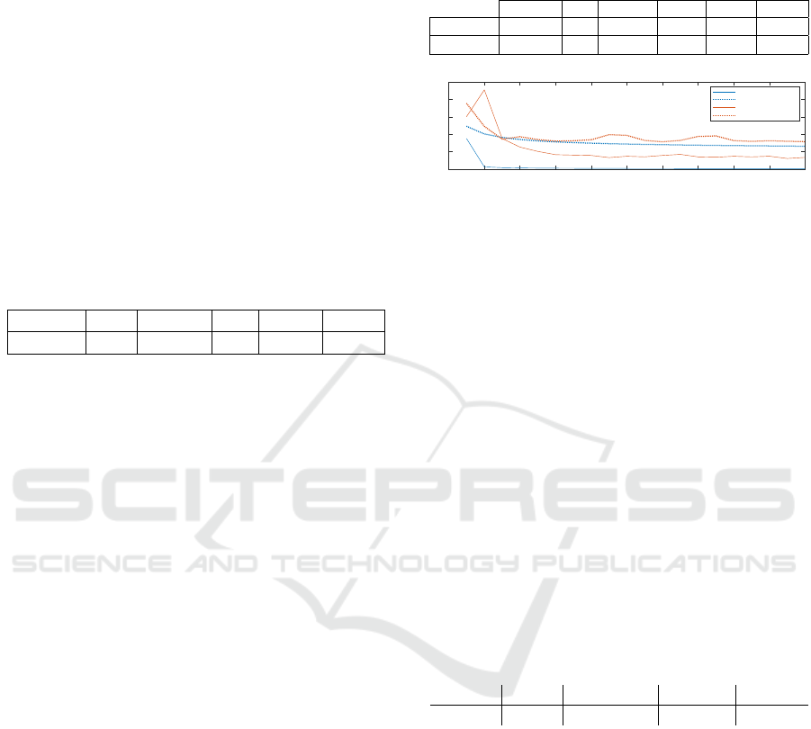
best, see Table 3. The amount of epochs was kept
to 20 to show that there was no substantial change in
later epochs. As it turns out, the training length could
be kept to approximately six epochs.
Table 3: Training parameters for the respective networks
BS = Batch Size, LR = Learning Rate, DS = Decay Speed,
Mom = Momentum.
Epochs BS LR DS Mom Loss
VGG19: 20 24 0.0001 0 0 MSE
ResNet: 20 24 0.0001 10
−6
0.9 MAE
0 2 4 6 8 10 12 14 16 18 20
Epochs
0
0.5
1
1.5
2
2.5
Mean Squared Error
Performance during training procedure
VGG19 - Training
VGG19 - Validation
ResNet50 - Training
ResNet50 - Validation
Figure 15: Comparison of performance between VGG19
and ResNet50 for the dataset containing faces only.
During training, augmentation methods, such as flip-
ping the image, were tested. No significant improve-
ment in performance was gained, so augmentation
was not used for training the networks. To keep the
original aspect ratio of the image when inputting the
image to the CNN, zero padding was tested before re-
sizing. This, however, led to a slight decrease in per-
formance, and was therefore not used during training.
3 RESULTS
3.1 Using Face Regions as Input
In this section, all methods were trained and tested on
cropped out faces only. The results for testing on the
standard test set are shown in Table 4.
Table 4: Mean absolute error for the standard test set con-
taining faces only.
Model: SVM Histogram VGG19 ResNet
MAE: 0.496 0.498 0.566 0.726
In Table 5, the performance of the different meth-
ods can be seen when tested on the stress test set.
Cells marked in green are considered acceptable and
cells marked with red are unacceptable. We allow a
deviation of 1 EV, due to the subjective assessment of
the test set.
All methods performed well on both test sets, ex-
cept for ResNet, which is lagging behind. It is notable
that Histograms actually perform better on the stress
test set than on the standard test set. It is also some-
what surprising that both CNN-based methods actu-
ally perform worse than the much simpler methods.
VISAPP 2021 - 16th International Conference on Computer Vision Theory and Applications
252
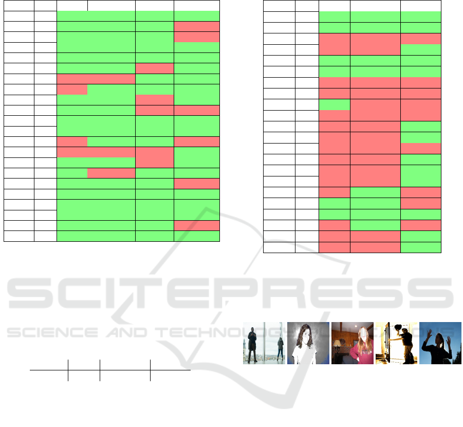
Table 5: Overview of the deviation from ground truth for
every test sample in the cropped stress test set.
IMG GT SVM Histogram VGG19 ResNet50
#1 2 0.22 0.06 0.95 0.17
#2 -2 0.86 0.87 0.34 1.45
#3 -1 0.43 0.37 0.44 1.60
#4 0 0.29 0.16 0.53 0.09
#5 -2 0.8 0.96 0.39 0.90
#6 2 0.46 0.64 1.33 0.71
#7 0 1.17 1.09 0.75 0.18
#8 0 1.25 0.09 0.16 0.42
#9 3 0.69 0.29 1.87 0.61
#10 3 0.49 0.32 1.72 1.24
#11 0 0.26 0.11 0.16 0.69
#12 0 0.6 0.69 0.84 0.35
#13 -2 1.21 0.62 0.05 1.94
#14 1 1.53 1.09 1.55 0.47
#15 0 0.54 0.44 1.61 0.71
#16 -1 0.64 1.22 0.25 0.23
#17 -2 0.28 0.02 0.49 3.04
#18 0 0.16 0.51 0.80 0.72
#19 0 0.06 0.11 0.09 0.51
#20 0 0.0 0.05 0.07 0.56
#21 0 0.68 0.02 0.44 1.55
MAE 0.601 0.468 0.707 0.863
3.2 Using Entire Photo as Input
In this test we leave out ResNet, as it performed the
worst on the faces-only test. The results can be seen
in Table 6 and Table 7
Table 6: Mean absolute error for the standard test set con-
taining the entire photos.
Model: SVM Histogram VGG19
MAE: 0.702 0.766 1.560
Looking at the standard test set, the two simple
methods perform better than the CNN, and this time
by quite a margin. This advantage, however, shifts
towards the CNN when it comes to the second test set
used for stressing the models. This probably means
that the CNN has learned where to look in the input
images. This was exactly the reason for employing
CNNs in the first place: The two other methods have
no spatial awareness and are forced to evaluate the
pictures as a whole. In many of the edge cases that
approach will fail, when we are specifically looking
for good exposure on faces.
4 DISCUSSION
The performance of all methods is good when evalu-
ating on the cropped dataset. The simple methods per-
form slightly better than the CNNs, but all are within
Table 7: Overview of the deviation from ground truth for
every test sample in the full-picture stress test set.
IMG GT SVM Histogram VGG19
#1 2 0.38 0.48 0.82
#2 -2 0.84 0.42 0.64
#3 -1 3.03 3.09 3.49
#4 0 2.35 2.3 0.82
#5 -2 0.66 0.58 0.57
#6 2 0.63 0.96 0.21
#7 0 2.45 2.79 1.62
#8 0 2.57 2.43 1.03
#9 3 2.33 1.32 2.17
#10 3 3.37 3.18 3.89
#11 0 2.35 1.03 0.73
#12 0 2.49 2.35 0.99
#13 -2 4.43 4.46 3.51
#14 1 1.77 1.46 0.32
#15 0 1.64 1.21 0.30
#16 -1 1.91 1.76 0.31
#17 -2 1.08 0.81 2.32
#18 0 0.39 0.21 1.11
#19 0 0.19 0.27 0.69
#20 0 1.18 0.95 1.25
#21 0 2.37 2.7 0.79
MAE 1.83 1.656 1.493
±1 EV
c
. Furthermore, this paper shows great poten-
tial in the use of CNNs for intelligent exposure esti-
mation, when looking at entire photographs. Here we
saw that the CNN did perform better than the other
two methods in the case of the stress test set. From
(a) #3 (b) #9 (c) #10 (d) #13 (e) #17
Figure 16: Overview of the images that did cause problems
in the network.
this test it can be seen that the CNN is more flexible
and dynamic than the other methods. This might be
due to the fact, that the CNN is able to look at differ-
ent areas of the image and does not use every single
pixel in the estimation, where the other models take
all the pixels into consideration.
The photographs which cause the largest errors
in the stress test set (see Fig. 16), are photographs
which are included to stress the model. These are
photographs where the exposure of the faces and the
background differ substantially, e.g in Fig. 16c, where
the background is exposed normally but the face is in-
deed overexposed. This indicates that the network is
capable of estimating the exposure level of a photo-
graph, but it does not always use the face as reference
for the estimation.
Facial Exposure Quality Estimation for Aesthetic Evaluation
253

To further explore the potential of using CNN for
this task, we dig into explainable AI, i.e. being able
to explain what the CNN is looking for in the image.
We analysed the results using LIME (Ribeiro et al.,
2016)
4
. Some of the results from the test with LIME
are shown in Fig. 17. As seen in Fig. 17, the net-
(a) 0.32 (b) 1.11 (c) 2.32 (d) 0.73 (e) 3.89
Figure 17: Overview of the results from Table 7, where the
deviation from ground truth is noted in the caption. The
regions highlighted in red are the parts that are used for the
estimates.
work uses the faces for estimates in some cases, while
in others it uses the face and other parts of the pho-
tograph. How close the estimation comes to ground
truth is in large part determined by whether non-face
parts of the photograph is used for the estimation.
Where it is found that if the face is not used for the
estimation at all, it deviates further from the ground
truth. This shows the the idea is solid, but the network
does not in its current iteration perform consistently,
and hence more data is needed for training to make
the network better at focusing on the relevant parts of
the images.
To solve that, one might look at fully training the
CNN on some other data sets other than ImageNet
to test whether an increase in the estimation quality
could be obtained. Here an interesting database could
be AVA, which is used for aesthetic image quality
analysis.
Pretraining on an aesthetic dataset might find
other deep features in the convolutional layers of the
network, than training on object classification. These
features might prove to be more beneficial for the
purpose of exposure estimation. Using weights pre-
trained on ImageNet might introduce brightness in-
sensitivity, which is perfect for object recognition, but
might not be beneficial for aesthetic evaluation, such
as exposure level.
5 CONCLUSION
In this paper, we have examined different methods for
exposure quality estimation of photographs. We focus
on exposure of faces, as most aesthetically pleasing
photos with people require good exposure in the face
region. This could be used to assist photographers in
4
https://github.com/marcotcr/lime
culling photographs, among other things. CNN-based
estimation has been compared to simpler regression
models based on handcrafted features and histograms,
respectively.
If we extract the faces before applying the meth-
ods, we were able to score an MAE of 0.707 using
VGG19. The simpler features outperformed the CNN
model. Both handcrafted features on pixel intensities,
and a neural network trained with histograms as input
performed well. In more complex scenes with dif-
ferent exposure levels across the image, the network
trained on histograms outperformed both other meth-
ods with a MAE of 0.468 compared to 0.601 for hand-
crafted and 0.707 for VGG19.
Looking at an entire photograph, the handcrafted
features and the histogram method perform better
than the CNN in simple situations, but when scenes
become complex, the handcrafted features are almost
useless. Here, the CNN model shows its potential,
due to its dynamic structure. Here an MAE of 1.83
was obtained for the handcrafted features and 1.656
for the histogram, where in the MAE for the CNN
stayed almost the same on 1.493.
Table 8: Recap of the results obtained for the second testset.
Cells in gray indicates only the face is used and cells in
white indicates the entire photo is used.
Method HC Hist VGG HC Hist VGG
MAE 0.601 0.468 0.707 1.83 1.656 1.493
There is room for improvement of the CNN, in order
to make sure it uses the face as reference for the ex-
posure measurement, but the network is able to esti-
mate the overall exposure of a photograph better than
handcrafted features. As mentioned in Section 1.2,
the localisation of focus within a photograph, is of
special importance too, and research within the use of
CNN’s for focus localisation is highly interesting in
the field of AI-assisted culling of photos. Future work
should include the creation of an extensive dataset
containing more diverse photographs, to catch several
photographic styles, such as high- and low-key pho-
tographs. This is needed in order to teach the neural
network to find and use the faces of the persons as
reference for the estimation.
The main findings of this paper is that models
based on handcrafted features or histograms outper-
form CNNs in the case of simple scenes. However,
when it comes to more complicated scenes, training
a CNN to estimate the exposure shows promise. In
most cases it seems that it is more prudent to use
handcrafted features in the case of estimating expo-
sure level, despite this, the use of CNNs for exposure
level estimation cannot be entirely ruled out.
VISAPP 2021 - 16th International Conference on Computer Vision Theory and Applications
254

ACKNOWLEDGEMENTS
We would like to thank Capture One for their contri-
butions to this paper. In particular Sune R. Bahn, Ines
Carton, Christian Gr
¨
uner, Claus Tørnes, and Hans J.
Skovgaard for providing insights into the field of pro-
fessional photography.
REFERENCES
Bianco, S., Celona, L., and Schettini, R. (2018). Aesthet-
ics assessment of images containing faces. 2018 25th
IEEE International Conference on Image Processing
(ICIP).
Chollet, F. et al. (2015). Keras. https://keras.io.
Datta, R., Joshi, D., Li, J., and Wang, J. Z. (2006). Studying
aesthetics in photographic images using a computa-
tional approach. European Conference on Computer
Vision.
Deng, Y., Loy, C. C., and Tang, X. (2017). Image aesthetic
assessment: An experimental survey. IEEE Signal
Processing Magazine, 34(4):80–106.
Dhar, S., Ordonez, V., and Berg, T. L. (2011). High level
describable attributes for predicting aesthetics and in-
terestingness. In CVPR 2011, pages 1657–1664.
Guo, L., Xiong, Y., Huang, Q., and Li, X. (2014). Image
esthetic assessment using both hand-crafting and se-
mantic features. Neurocomputing, 143:14–26.
He, K., Zhang, X., Ren, S., and Sun, J. (2015). Deep
residual learning for image recognition. CoRR,
abs/1512.03385.
Kao, Y., Huang, K., and Maybank, S. (2016). Hierarchical
aesthetic quality assessment using deep convolutional
neural networks. 47:500–511.
Ke, Y., Tang, X., and Jing, F. (2006). The design of high-
level features for photo quality assessment. IEEE
Computer Society Conference on Computer Vision
and Pattern Recognition.
Li, C., Gallagher, A., Loui, A. C., and Chen, T. (2010).
Aesthetic quality assessment of consumer photos with
faces. International Conference on Image Processing.
Lu, X., Lin, Z., Jin, H., Yang, J., and Wang, J. Z. (2014).
Rapid: Rating pictorial aesthetics using deep learning.
Marchesotti, L., Perronnin, F., Larlus, D., and Csurka, G.
(2011). Assessing the aesthetic quality of photographs
using generic image descriptors. International Con-
ference on Computer Vision.
Murray, N., Marchesotti, L., and Perronnin, F. (2012). Ava:
A large-scale database for aesthetic visual analysis.
pages 2408–2415.
Obrador, P., Schmidt-Hackenverg, L., and Oliver, N. (2010).
The role of image composition in image aesthetics.
International Conference on Image Processing.
Ribeiro, M., Singh, S., and Guestrin, C. (2016). “why
should i trust you?”: Explaining the predictions of any
classifier. pages 97–101.
Simonyan, K. and Zisserman, A. (2014). Very deep convo-
lutional networks for large-scale image recognition.
Tian, X., Dong, Z., Yang, K., and Mei, T. (2015). Query-
dependent aesthetic model with deep learning for
photo quality assessment. IEEE Transactions on Mul-
timedia, 17:1–1.
Tong, H., Li, M., Zhang, H.-J., He, J., and Zhang, C. Clas-
sification of digital photos taken by photographers or
home users.
Facial Exposure Quality Estimation for Aesthetic Evaluation
255
