CPA Lyapunov Functions: Switched Systems vs. Differential Inclusions

Sigurdur Hafstein

Science Institute and Faculty of Physical Sciences, University of Iceland, Dunhagi 5, 107 Reykjav

ık, Iceland

Keywords:

Lyapunov Function, Switched Systems, Differential Inclusions, Numerical Algorithm, Artstein’s Circles.

Abstract:

We present an algorithm that uses linear programming to parameterize continuous and piecewise afﬁne Lya-

punov functions for switched systems. The novel feature of the algorithm is, that it can compute Lyapunov

functions for switched system with a strongly asymptotically stable equilibrium, for which the equilibrium of

the corresponding differential inclusion is merely weakly asymptotically stable. For the differential inclusion

no such Lyapunov function exists. This is achieved by removing constraints from a linear programming prob-

lem of an earlier algorithm to compute Lyapunov functions, that are not necessary to assert strong stability for

the switched system. We demonstrate the beneﬁts of this new algorithm sing Artstein’s circles as an example.

1 INTRODUCTION

We start with an informal introduction of the switched

systems and differential inclusions we will be con-

cerned with; the technical details follow later when

we concretize our setting. Keep in mind that we are

setting the stage to remove conditions on a Lyapunov

function for a switched system with a strongly asymp-

totically stable equilibrium, which is merely weakly

asymptotically stable for the corresponding differen-

tial inclusion.

We consider switched systems of the form

x = f

(x), α : [0, ∞) → A, (1)

where for each a ∈ A the vector ﬁeld f

: D(f

) → R

is deﬁned on D(f

) ⊂ R

, A is a ﬁnite set equipped

with the discrete topology, and α : [0, ∞) → A is a

right-continuous switching signal. Solution trajecto-

ries of the system are continuous paths obtained by

gluing together trajectory pieces of the individual sys-

tems

x = f

(x). Switched systems and their stabil-

ity have been intensively studied, cf. the monograph

(Liberzon, 2003; Sun and Ge, 2011). The main ques-

tions regarding the asymptotic stability of an equilib-

rium of a switched system, which we may assume is at

the origin, is if a switching can be chosen such that so-

lution trajectories are steered to the equilibrium (weak

asymptotic stability) or if trajectories are attracted to it

regardless of the switching (strong asymptotic stabil-

ity). The latter case is referred to as arbitrary switch-

ing. Both types of stability are usually dealt with us-

ing Lyapunov functions, i.e. functions from the state

space to the real numbers that are decreasing along so-

lution trajectories. In (Hafstein, 2007) an algorithm to

compute continuous and piecewise afﬁne (CPA) Lya-

punov functions for arbitrary switched systems was

developed; we will discuss it below.

Closely related to the switched system (1) is the

differential inclusion

x ∈ F(x) := co{f

(x) : x ∈ D(f

)}, (2)

where coC denotes the convex hull of the set C ⊂ R

Solution trajectories are absolutely continuous paths

t 7→ x(t) fulﬁlling

x(t) ∈ F(x(t)) almost surely. One

speaks of weak asymptotic stability of an equilibrium

if there are solution trajectories that are asymptot-

ically attracted towards the equilibrium and strong

asymptotic stability if this is the case for all solu-

tion trajectories. In (Baier et al., 2010; Baier et al.,

2012) an algorithm for the computation of CPA Lya-

punov functions for strongly asymptotically stable in-

clusions was presented and in (Baier and Hafstein,

2014) a corresponding algorithm for the computa-

tion of control CPA Lyapunov functions for weakly

asymptotically stable differential inclusions. See also

(Baier et al., 2018) for a different approach including

semiconcavity condition into the formulation of the

optimization problem.

Let us give a short review of CPA Lyapunov func-

tions in the context of switched systems and differ-

ential inclusions. To deﬁne a CPA Lyapunov func-

tion V , ﬁrst a triangulation T of its domain, a subset

of R

, must be ﬁxed. The triangulation must have

the property that any two different simplices inter-

sect in a common face or not at all. The continuous

Hafstein, S.

CPA Lyapunov Functions: Switched Systems vs. Differential Inclusions.

DOI: 10.5220/0009992707450753

In Proceedings of the 17th International Conference on Informatics in Control, Automation and Robotics (ICINCO 2020), pages 745-753

ISBN: 978-989-758-442-8

745

and piecewise afﬁne function V is then deﬁned by as-

signing it values at the vertices of the simplices of T

and linearly interpolating these values over the sim-

plices. The resulting function is afﬁne on each sim-

plex S

∈ T and thus differentiable in its interior S

◦

In particular, its gradient is a well deﬁned constant

vector ∇V

in the interior. At the boundaries, where

two or more simplices intersect, the function V is not

differentiable and its gradient is not deﬁned. In (Baier

et al., 2010; Baier et al., 2012; Baier and Hafstein,

2014) this was dealt with in the context of nonsmooth

analysis using the Clarke subdifferential, which can

be deﬁned through

∂

V (x) := co{ lim

→x

∇V(x

) : ∃ lim

→x

∇V(x

)} (3)

for locally Lipschitz continuous V , cf. (Clarke, 1990).

That is, Clarke’s subdifferential ∂

V (x) ⊂ R

is the

convex hull of all converging sequences (∇V (x

))

i∈N

where x

→ x as i → ∞. The establishing of the strong

stability of an equilibrium of the differential inclusion

(2) now essentially boils down to showing, where

•

denotes the dot product of vectors and sets of vectors

•

M := {x

•

y : x ∈ N,y ∈ M}, that

∂

V (x)

•

F(x) < 0 (4)

in a punctuated neighbourhood of the equilibrium. In

this context < means that every element of the set on

the left-hand side is less than zero. For a CPA function

V this further simpliﬁes to

∇V

•

(x) < 0 (5)

for every ν such that x ∈ S

and every a ∈ A such that

x ∈ D(f

). This comes as every element in ∂

V (x)

is the convex sum of such ∇V

and every element of

F(x) is the convex sum of such f

(x). Exactly the

same condition (5) can be used to show the strong sta-

bility of the same equilibrium for the switched system

(1).

Now, even for considerably more general differ-

ential inclusions than (2), i.e. compact, convex, upper

semicontinuous F, the strong asymptotic stability of

an equilibrium was shown in (Clarke et al., 1998) to

be equivalent to the existence of a Lyapunov function

V fulﬁlling (4). However, there are arbitrary switched

systems with a strongly asymptotically stable equilib-

rium, such that the equilibrium is only weakly sta-

ble for the corresponding differential inclusion. We

will modify the CPA algorithm to compute Lyapunov

functions for arbitrary switched system and differen-

tial inclusions to deal with this case. Our motivating

example will be that of Artstein’s circles.

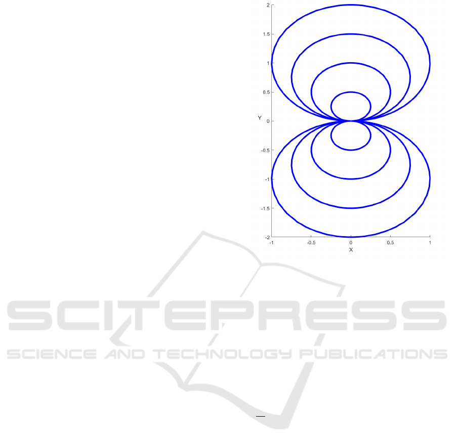
Figure 1: Trajectories of Artstein’s circles (6). For an initial

value (x

) the trajectory is an arc of a circle with center

on the y-axis and passing through (0,0) and (x

). Vary-

ing u changes the speed and the orientation of how the cir-

cles are traversed. For u > 0 the upper circles are traversed

clockwise and the lower circles counter-clockwise until the

equilibrium at zero is reached; for u < 0 vise versa. The

speed of the traversing is proportional to |u|.

1.1 Artsteins’s Circles

Artstein’s circles (Artstein, 1983) are given by the dif-

ferential inclusion





∈





−x

+ y

−2xy



: u ∈ [−1, 1]



. (6)

See Fig. 1 for its solution trajectories. Clearly, the

equilibrium at zero is not strongly asymptotically sta-

ble for the differential inclusion, ﬁx e.g. u = 0. How-

ever, it is clearly weakly stable because, e.g. ﬁxing

u = −1 or u = 1, delivers an ODE with this property.

Let us deﬁne

(x,y) =



−x

+ y

2xy



(7)

and f

−

(x,y) = −f

(x,y). Then system (6) can be

written

x ∈ co{f

−

(x),f

(x)} and the corresponding

switched system is

x = f

(x), α : [0, ∞) → {−, +}, (8)

for which the origin is a weakly asymptotically stable

equilibrium, and not strongly asymptotically stable!

From now on we limit the domains of f

−

and

to D(f

−

) = (−∞,0] × R and D(f

) = [0,∞) × R.

ICINCO 2020 - 17th International Conference on Informatics in Control, Automation and Robotics

746

Then the switched system (8) has a strongly asymp-

totically stable equilibrium at the origin. The reason

for this is that the switching only has more than one

option on D(f

−

) ∩ D(f

) = {0} × R, and no mat-

ter which choice is made, the system state is asymp-

totically attracted to the origin. The decision only

inﬂuences whether the left- or the right trajectory

arc is traversed. Note that for the inclusion

x ∈

co{f

−

(x),f

(x)} with these domains for f

−

(x) and

(x), the origin is weakly- but not strongly asymptot-

ically stable, because 0 ∈ co{f

−

(x),f

(x)} for every

x ∈ {0} × R.

It follows from the discussion above, that there

does not exists a CPA Lyapunov function V fulﬁlling

(5) for the switched system (8), although the equilib-

rium is strongly asymptotically stable. The condition

(5) is unnecessary strict for switched systems; it is

used to assert

limsup

h→0+

V (x + hf

(x)) −V (x)

< 0 (9)

for all f

such that x ∈ D(f

), but this may hold true

although (5) fails for some of them. To see this con-

sider two triangles, S

= co{(−c, c), (0, c), (0,2c)}

and S

= co{(c,c), (0, c), (0, 2c)} for c > 0, and x =

(0,3c/2) for the switched system (8). Let V be a CPA

function such that ∇V

•

−

(x) < 0 and ∇V

•

(x) < 0.

Since f

−

(x) = −f

(x) this implies ∇V

•

(x) > 0 and

∇V

•

−

(x) > 0, but (9) still holds true. The reason is

that f

−

(x) points into S

and f

(x) points into S

. In

our modiﬁed CPA algorithm below we systematically

remove such unnecessary constraints from the origi-

nal linear programming problem.

2 THE SETUP

For formulating our modiﬁed CPA algorithm for

switched system some preparation is needed. Let

{

}

ν∈T

= T , T an index set, be a set of simplices

in R

, such that different simplices S

∈ T inter-

sect in a common face or not at all and with D

ν∈T

, D

◦

is a simply connected neighborhood of

the origin. The set T is the triangulation that we use

to deﬁne a CPA function V by ﬁxing its values at the

vertices

:= {x

: x

is a vertex of a simplex S

∈ T }

of the triangulation.

For each S

∈ T denote by C

= {x

,...,x

}

the set of its vertices. Thus S

= coC

and S

∩ S

co(C

∩C

). Deﬁne I

: R

⇒ T by I

(x) := {ν ∈

T : x ∈ S

}. Thus I

(x) is a set of the indices of the

simplices in T containing x. The notation ⇒ denotes

a multivalued function, the values of I

are subsets

of T . We consider arbitrary switched systems as (1)

and corresponding differential inclusions (2) that are

adapted to the triangulation T .

For deﬁning what adapted to the triangulation T

means some further deﬁnitions are useful: Let A be

a ﬁnite set and f

: D(f

) → R

be vector ﬁelds, such

that for every a ∈ A the domain D(f

) ⊂ R

of f

the union of some of the simplices in T . Thus, for

every a ∈ A we have

0 6= D(f

) = S

∪S

∪· ··∪ S

where ν

,ν

,...,ν

∈ T . Deﬁne for every ν ∈ T the

set

:= {a ∈ A : S

⊂ D(f

)}

and assume that A

0 for all ν ∈ T . Hence, on every

simplex S

∈ T at least one of the vector ﬁelds f

deﬁned.

For a simplex S

∈ T deﬁne the set

:= {S

∈ T : S

6= S

and S

∩ S

of its neighbouring simplices in T .

Our modiﬁed CPA algorithm will eliminate un-

necessary constraints from the original linear pro-

gramming problem. For this we need to deﬁne for

every simplex S

and every vector ﬁeld f

deﬁned on

the simplex S

, i.e. every a ∈ A

, the set of the essen-

tial neighbouring simplices ENS

with respect to the

vector ﬁeld f

. That is, ENS

contains the simplices

∈ NS

, such that solution trajectories of

x = f

(x)

with an initial position in x ∈ S

can move into the

interior of S

in an inﬁnitesimal time. In formula, for

every S

∈ T and every a ∈ A

deﬁne

ENS

:= {S

∈ NS

: ∃x ∈ S

, ∃h > 0

s.t. x + [0,h]f

(x) ⊂ S

where

x + [0,h]f

(x) := {x + h

(x) : 0 ≤ h

≤ h}.

Deﬁne

V (x, y) := lim sup

h→0+

V (x + hy) −V (x)

It is well known that D

V (x, f

(x) is the orbital

derivative of a locally Lipschitz V at point x along

the solution trajectories of

x = f

(x), i.e. if t 7→ φ(t) is

the solution with φ(0) = x, then

V (x, f

(x)) = lim sup

h→0+

V (φ(h)) −V (x)

for a proof cf. e.g. (Marin

osson, 2002, Th. 1.17). Fur-

ther, CPA functions are obviously locally Lipschitz.

Lemma 2.1. For every S

∈ T such that there ex-

ists an h > 0 with x + [0, h]f

(x) ⊂ S

we have

V (x, f

(x)) = ∇V

•

(x).

CPA Lyapunov Functions: Switched Systems vs. Differential Inclusions

747

Proof. Assume x + [0,h]f

(x) ⊂ S

∩ S

for two sim-

plices S

∈ T . Since V is afﬁne on both simplices

and S

we have for some constants a

∈ R and

∇V

and ∇V

deﬁned as above that V (y) = ∇V

•

y +

for all y ∈ S

and V (y) = ∇V

•

y+a

for all y ∈ S

In particular, we have for all y ∈ S

∩ S

that

∇V

•

y + a

= ∇V

•

y + a

Now substitute x + h

(x) for y and simplify to get

(∇V

− ∇V

)

•

(x) = a

− a

− (∇V

− ∇V

)

•

and note that this equation must hold true for all 0 ≤

≤ h. Since the right-hand side is constant we must

have (∇V

− ∇V

)

•

(x) = 0. The statement is now

obvious.

The next lemma justiﬁes the nomenclature for

ENS

: essential neighbouring simplices with respect

to the vector ﬁeld f

Lemma 2.2. Let x ∈ D

◦

. Then there is a ν ∈ T such

that x ∈ S

and for every a ∈ A

we have

V (x, f

(x)) = ∇V

•

(x) (10)

where µ = ν or S

∈ ENS

Proof. That there is a ν ∈ T such that x ∈ S

follows

directly from our setup. Since simplices are convex

and closed there surely exists an h > 0 and µ ∈ T such

that x+ [0, h]f

(x) ⊂ S

and by the deﬁnition of ENS

necessarily S

∈ ENS

if µ 6= ν.

3 THE MODIFIED

CONSTRAINTS

We now describe how we eliminate unnecessary con-

straints from the liner programming problem in (Baier

and Hafstein, 2014). Note that this is the same linear

programming problem as for the differential inclusion

in (Baier et al., 2010; Baier et al., 2012), but when the

differential inclusion is considered, then these con-

straints are necessary. Indeed, as discussed in Sec-

tion 1.1 for Artstein’s circles, the equilibrium might

be merely weakly asymptotically stable for the differ-

ential inclusion, although it is strongly asymptotically

stable for the corresponding switched system.

The constraints to enforce ∇V

•

(x) < 0 for all

x ∈ S

are only veriﬁed at the vertices of the simplex

. As a consequence one must verify ∇V

•

) <

−a

at the vertices x

of the simplex S

for appropriate

> 0, to make sure that the inequality folds for all

x ∈ S

. This motivates the following deﬁnitions.

For a set C = {x

,...,x

} of afﬁnely indepen-

dent vectors in R

and a vector ﬁeld f

deﬁned on coC

with components ( f

, f

,..., f

) = f

deﬁne

C,r,s

:= max

x∈coC

m=1,2,...,n



∂

∂x

(x)



. (11)

Further, for each (vertex) y ∈ C deﬁne

max

y,s

:= max

j=0,1,...,k

•

− y)|

and let E

a,y

C,x

, i = 0, 1,...,k, be constants such that

a,y

C,x

≥ (12)

∑

r,s=1

C,r,s

•

− y)|(C

max

y,s

+ |e

•

− y)|).

A few comments are in order. As shown later,

the constants E

a,y

C,x

are deﬁned such that if for one

ﬁxed vertex y of the simplex S

= coC

∈ T , C

,...,x

}, we have

∇V

•

) < −E

a,y

C,x

k∇V

, i = 0, 1,...,k = n,

then ∇V

•

(x) < 0 for all x ∈ S

For implementing the constraints it is of essen-

tial practical importance that E

a,y

C,x

is an upper bound,

which in effect means that one must not compute

the B

C,r,s

exactly, which can be difﬁcult. Any upper

bound on the second order derivatives of the com-

ponents f

can be used. However, less conservative

bounds might mean that one needs smaller simplices

to fulﬁll the constraints.

Finally, if

a,y

C,x

≥ h

∑

r,s=1

C,r,s

whith h

= diam(C) := max

x,y∈C

kx − yk

, then the

estimate (12) follows. In particular one can for sim-

plicity use a uniform bound

≥ max

x∈D(f

)

m,r,s=1,2,...,n



∂

∂x

(x)



and set E

a,y

C,x

= n

, where h

:= diam(S

), for

0 6= C ⊂ C

. Indeed, a little more careful analysis us-

ing that kxk

≤ nkxk

shows that using

a,y

C,x

= nB

is enough to fulﬁll the estimate (12), cf. e.g. (Baier

et al., 2012). However, although this more conserva-

tive formula is more pleasant to the eye, the imple-

mentation of (12) is not more involved in practice.

We therefore use the sharper estimate (12) in what

ICINCO 2020 - 17th International Conference on Informatics in Control, Automation and Robotics

748

follows. Note, however, that in order to understand

the linear programming problems very little is lost if

one just considers the E

a,y

C,x

as appropriate constants

needed to interpolate inequality conditions from ver-

tices over simplices and faces and of simplices, with-

out following the details. Computing the E

a,y

C,x

al-

gorithmically is simple given some upper bounds on

the second order derivatives of the components of the

vector ﬁelds f

We are now ready to state our linear programming

problem to compute CPA Lyapunov functions. We

ﬁrst state it as in (Baier et al., 2010; Baier et al., 2012)

and then outline a proof of why a feasible solution to it

delivers a CPA Lyapunov function for the differential

inclusion used in its construction. From the proof it

becomes clear what conditions are unnecessary when

we move from the differential inclusion (2) to the ar-

bitrary switched system (1). In Section 3.2 we then

discuss how the removing of constraints can be algo-

rithmically implemented.

3.1 The Linear Programming Problem

Consider a triangulation T as in Section 2 and,

adapted to the triangulation, the differential inclusion

(2) and the corresponding arbitrary switched system

(1). Assume that the equilibrium in question is at the

origin. For every simplex S

∈ T let

= {x

,...,x

}

denote its vertices, i.e. S

= coC

. Assume that for

every S

= coC

∈ T and every

0 6= C ⊂C

and every

a ∈ A

we have an upper bound B

C,r,s

as in (11) and

that we have ﬁxed a vertex y of C for the deﬁnition

of E

a,y

C,x

. If 0 ∈ C we must choose y = 0 to avoid un-

satisﬁable constraints. Note that the sets coC, where

0 6= C ( C

, are the faces of the simplex S

The variables of the linear programming problem

are V

for every x that is a vertex of a simplex in T ,

i.e. x ∈ V

. From a feasible solution, where the vari-

ables V

have been assigned values such that the lin-

ear constraints below are fulﬁlled, we then deﬁne a

continuous function V : D

→ R through parameteri-

zation using these values: for an x ∈ D

we can ﬁnd a

simplex S

= co{x

,...,x

} such that x ∈ S

and x

has a unique representation x =

∑

i=0

as a convex

sum of the vertices. For x we deﬁne

V (x) :=

∑

i=0

If two different simplices in T intersect they do so in

a common face, hence V is well-deﬁned and continu-

ous. By a slight abuse of notation we both write V (x

)

for the variable V

of the linear programming prob-

lem and the value of the function V at x

, since after

we have assigned a numerical value to the former it is

the value of the function V at x

There are two groups of constrains in the linear

programming problem. The ﬁrst group is to assert

that V has a minimum at the origin:

Linear Constraints L1

If 0 ∈ V

one sets V (0) = 0. Then for all x ∈ V

V (x) ≥ kxk

Another possibility is to relax the condition of

strong asymptotic stability of the origin to practical

strong asymptotic stability. In this case one prede-

ﬁnes an arbitrary small neighbourhood of the origin

N and does not demand that V is decreasing along

solution trajectories in this set. One must then make

sure through constraints that

max

x∈∂N

V (x) < min

x∈∂D

V (x),

because sublevel sets of V that are closed in D

◦

are

lower bounds on the basin of attraction. This is not

difﬁcult to implements and is discussed in detail in

e.g. (Hafstein, 2004; Hafstein, 2007; Baier et al.,

2012; Hafstein et al., 2015). In short, the implica-

tions of such a Lyapunov function are that solutions

enter N in a ﬁnite time and either stay in N or stay

close and enter it repeatedly.

The second group of linear constraints is to assert

that V is decreasing along all solution trajectories.

The simplest case is when A

= A for all ν ∈ T and

then the appropriate constraints are:

Linear Constraints L2 (Simplest Case)

For every S

∈ T , we demand for every a ∈ A

and

i = 0, 1,...,n that:

∇V

•

) + k∇V

a,y

≤ −kx

. (13)

In the case of practical strong asymptotic stabil-

ity one disregards the constraints (13) for S

⊂ N .

Note that the constrains (13) are linear in the vari-

ables V (x

), cf. e.g. (Giesl and Hafstein, 2014, Re-

marks 9 and 10), in particular k∇V

can be mod-

elled through linear constraint using auxiliary vari-

ables.

Now, let us consider how one uses the con-

straints (13) to show that D

V (x, f

(x)) ≤ −kxk

. By

(Marin

osson, 2002, Lemma 4.16) we have for a ∈ A

and x =

∑

i=0

∈ S

∑

i=0

= 1, that



(x) −

∑

i=0

)



∞

≤

∑

i=0

a,y

. (14)

CPA Lyapunov Functions: Switched Systems vs. Differential Inclusions

749

Hence, H

older inequality, constraints (13), and the

convexity of the norm imply that

∇V

•

(x) = (15)

∑

i=0

∇V

•

) + ∇V

•

(x) −

∑

i=0

)

≤

∑

i=0

∇V

•

) + k∇V

∑

i=0

a,y

∑

i=0



∇V

•

) + k∇V

a,y



≤

∑

i=0

(−kx

) ≤ −k

∑

i=0

= −kxk

For an x ∈ S

◦

we have the existence of an h > 0 such

that x + h

(x) ⊂ S

for all 0 ≤ h

≤ h and we get by

Lemma 2.2 that

V (f

(x),x) = ∇V

•

(x) ≤ −kxk

for all a ∈ A

. For an x ∈ ∂S

we cannot con-

clude this in general, because is is possible that x +

[0,h]f

(x) 6⊂ S

for any h > 0 and we need the con-

straints (13) to hold true with ν = µ, where S

is such

that x + [0,h]f

(x) ⊂ S

for some h > 0. Note that if

a ∈ A

then this is assured, therefore nothing can go

wrong if A

= A for all µ ∈ T .

In (Baier et al., 2010; Baier et al., 2012) the

general case, when A

6= A for some µ ∈ T , was dealt

with by adding the constraints:

Linear Constraints L2 (Old)

For every S

= coC

∈ T we demand for every a ∈

, in addition to the constraints (13), that for every

∈ NS

such that a /∈ A

we have for C = C

∩C

,...,x

} that:

∇V

•

) + k∇V

a,y

C,x

≤ −kx

(16)

for i = 0, 1,...,k.

Note that the linear constraints (16) imply by com-

putations analog to (15) that ∇V

•

(x) ≤ −kxk

for

every x ∈ D(f

), even if a /∈ A

, i.e. S

6⊂ D(f

) and

is only deﬁned on a face of S

. Just substitute n,

∇V

, x

, E

a,y

with k, ∇V

, x

, E

a,y

C,x

, respectively, in

the computations (15).

For the differential inclusion (2) these constraints

is indeed necessary to show strong asymptotic stabil-

ity of the equilibrium at the origin, or strong practical

asymptotic stability of a set N , because for a CPA

function V we have

∂

V (x) := co{∇V

: x ∈ S

}

and

F(x) = co{f

(x) : x ∈ D(f

(x))}.

Hence ∂

V (x)

•

F(x) ⊂ R consists of the elements

∑

µ:x∈S

∇V

•

∑

a:x∈D(f

)

(x)

∑

µ: x∈S

a: x∈D(f

)

∇V

•

(x),

for all α

,β

≥ 0 fulﬁlling

∑

µ:x∈S

∑

a:x∈D(f

(x))

= 1.

In the case S

⊂ D(f

), S

6⊂ D(f

), and x ∈ S

∩ S

we have S

∈ NS

and the constraints (16) assure that

∇V

•

(x) < −kxk

However, by Lemma 2.2, we can conclude

V (f

(x),x) ≤ −kxk

if the constraints (13) hold

for all essential neighbours S

∈ ENS

of S

with

respect to the vector ﬁeld f

. We do not need to

consider neighbouring simplices S

∈ NS

that are

not essential! The modiﬁed constraints are :

New Linear Constraints L2

For every S

= coC

∈ T we demand for every a ∈

, in addition to the constraints (13), that for every

∈ ENS

such that a /∈ A

we have for C = C

∩C

,...,x

} that:

∇V

•

) + k∇V

a,y

C,x

≤ −kx

(17)

for i = 0, 1,...,k.

Note that the only difference between the old con-

straints and the new ones is that NS

in the old ones

has been replaced by ENS

in the new ones.

For algorithmically implementing the new con-

straints we need to be able to generate the sets ENS

efﬁciently. In practice we can efﬁciently compute sets

(ENS

)

∗

⊂ (ENS

)

∗

⊂ ENS

using some of the same ideas as in the computa-

tions (15). The practical implementation of New lin-

ear constraints L2 is then done by using these sets

(ENS

)

∗

instead of the sets ENS

. We describe the

details of how to compute the sets (ENS

)

∗

in the next

section.

3.2 Computing Essential Neighbours

Consider a simplex S

= coC

∈ T , where as before



,...,x



. Another way to describe the

simplex S

is to deﬁne it as the intersection of n + 1

half-spaces. Recall that a half-space is deﬁned as {x ∈

: n

•

(x−y) ≥ 0} for some vectors n,y ∈ R

, n 6= 0.

ICINCO 2020 - 17th International Conference on Informatics in Control, Automation and Robotics

750

These half-spaces for S

can be constructed using the

set C

as follows, see also (Hafstein, 2017).

For i = 0,1, . . .,n we construct a half-space H

ν,x

such that S

⊂ H

ν,x

and C

\ {x

} is a subset of the

boundary ∂H

ν,x

of H

ν,x

in the following way:

Set y

:= x

and pick an arbitrary, but ﬁxed vector

∈ C

\ {x

}. Let {y

,...,y

n−1

} = C

\ {y

}

and deﬁne the matrix n × n matrix

ν,x

:= (y

− y

,...,y

− y

)

That is, the ﬁrst row in the matrix Y

ν,x

is the vector

− y

, the second row is the vector y

− y

, etc.

Because the vectors y

,...,y

are afﬁnely in-

dependent the matrix Y

ν,x

is non-singular and the

equation

ν,x

y = e

where e

is the usual n-th unit basis vector, has a

unique solution n

ν,x

for y. Deﬁne the half-space

ν,x

:= {x ∈ R

: n

ν,x

•

(x − y

) ≥ 0}. (18)

Note that H

ν,x

is a half-space such that S

⊂ H

ν,x

and the vertices y

,...,y

n−1

of the simplex S

, and

hence the face co(C

\ {x

}), are in the hyper-plane

∂H

ν,x

dividing the space. This can be seen from

ν,x

= Y

−1

ν,x

and then, since

ν,x

•

(x − y

) = e

−T

ν,x

(x − y

where Y

−T

ν,x



−1

ν,x



, and Y

−T

ν,x

(x − y

) = e

for

x = y

, k = 1, 2, . ..,n, we have n

ν,x

•

− y

) = 0 if

k = 1, 2, . . . ,n − 1 and n

ν,x

•

− y

) = 1.

Every point x ∈ S

can be written uniquely as a

convex combination x =

∑

k=0

and thus

x − y

∑

k=0

− y

Hence,

ν,x

•

(x − y

) = λ

from which the propositions follow. Using these re-

sults it is easily veriﬁed that

i=0

ν,x

. (19)

We now use this to compute a set (ENS

)

∗

such

that ENS

⊂ (ENS

)

∗

⊂ NS

. Fix an S

∈ NS

and

let

,...,z

} = C

∩C

and

,...,y

} = C

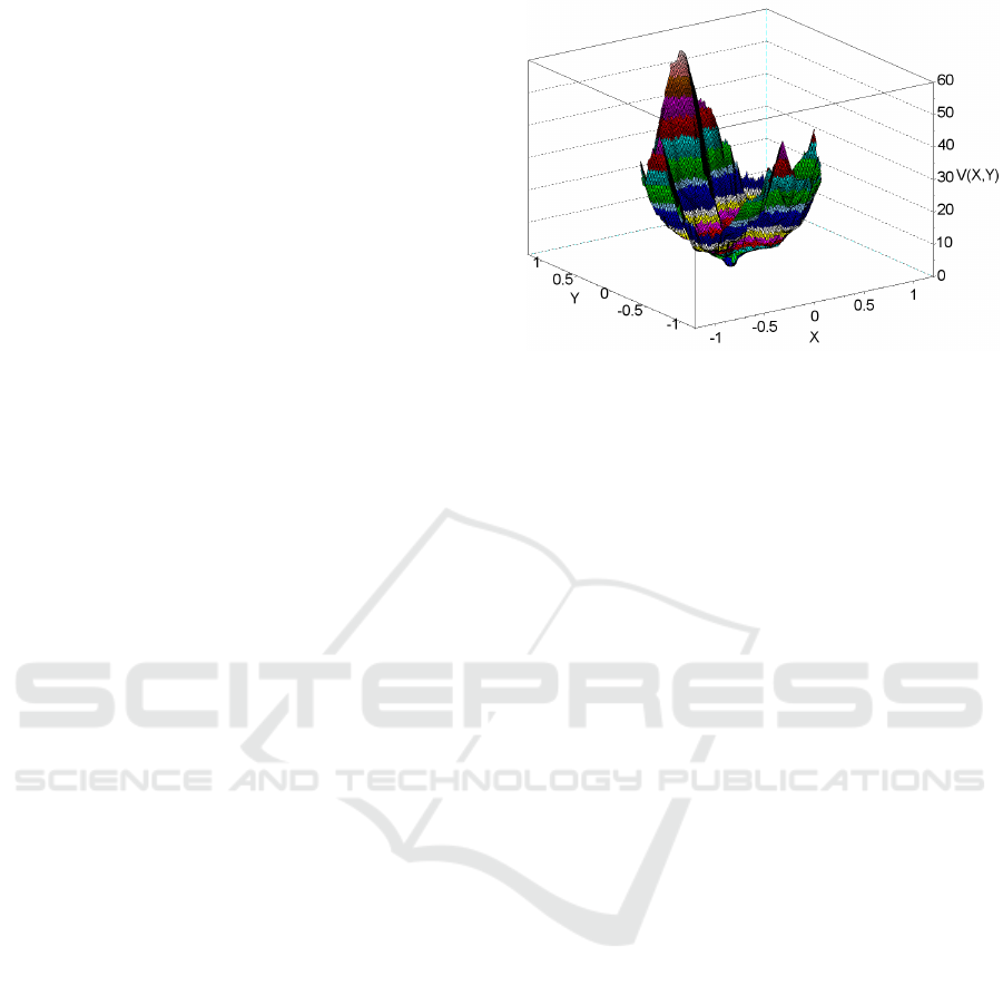
Figure 2: Continuous piecewise afﬁne Lyapunov function

computed for Artstein’s circles with the new algorithm.

Corresponding to the half-spaces H

µ,y

are the vectors

µ,y

computed as above, but now for the simplex S

and its vertices C

⊃ {y

,...,y

}. Assume that for

any j ∈ {1, 2, . ..,s} we have

0 > n

µ,y

•

) + E

a,y

∩C

µ,y

(20)

for all i = 1, 2,...,r. Then, for an arbitrary convex

combination x =

∑

i=1

, we have

µ,y

•

(x) =

∑

i=1

µ,y

•

)

+ n

µ,y

•

(x) −

∑

i=1

)

≤

∑

i=1



µ,y

•

) + E

a,y

∩C

µ,y



< 0.

In particular, because n

µ,y

•

(x − z

) = 0 as shown

above, where z

∈ C

∩C

corresponds to the vector

in (18), we have

µ,y

•

(hf

(x) + x − z

) = h



µ,y

•

(x)



< 0

for all h > 0. Hence, hf

(x)+ x /∈ H

µ,y

for any h > 0,

which, by (19), implies hf

(x) + x /∈ S

for any h > 0.

Thus S

/∈ ENS

For each a ∈ A

we deﬁne (ENS

)

∗

as those S

∈

that are not eliminated by this process. That is,

∈ (ENS

)

∗

if for all j = 1,2,..., s the inequality

(20) fails to hold true for at least one i ∈ {1,2,...,r}.

Note that this is easily checked algorithmically. For a

visual illustration of the sets (ENS

)

∗

see Fig. 3.

Returning to our example of Artstein’s circles,

this new algorithm easily generates a CPA Lyapunov

function for the system (8) in a few seconds after the

domains of f

and f

−

have been ﬁxed as D(f

−

) =

(−∞,0]× R and D(f

) = [0, ∞) × R, see Fig. 2. With

CPA Lyapunov Functions: Switched Systems vs. Differential Inclusions

751

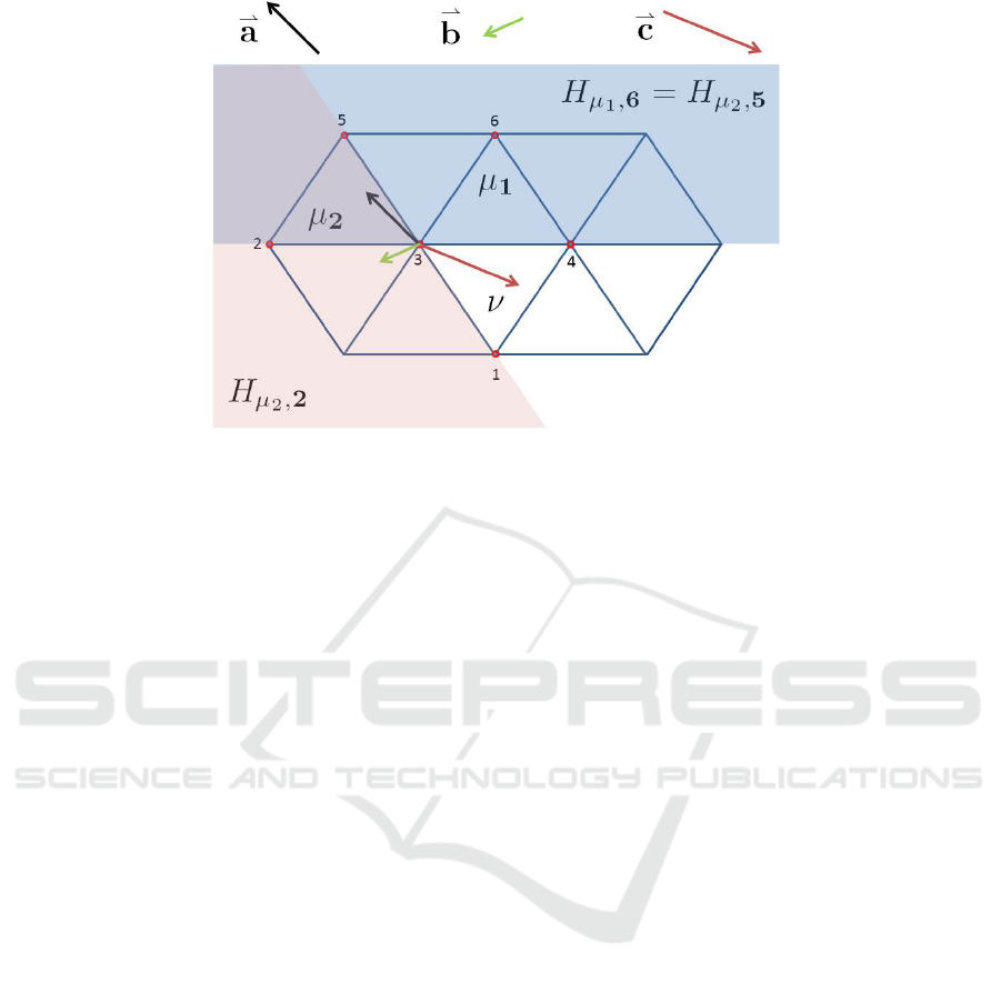
Figure 3: The simplex S

is the convex combination of the 3 = n+1 vertices 1,3,4, i.e. S

= co{1,3, 4}, and S

= co{3,4, 6},

and S

= co{2,3, 5}. Clearly {S

} ⊂ NS

. We consider three constant f

(x) on S

: f

(x) =

a , f

(x) =

b, and f

(x) =

c ;

depicted by arrows. Since the vector ﬁelds are constant the sets ENS

and (ENS

)

∗

coincide. Now S

∩ S

= co{3, 4} and

the half-space H

, with co{3,4} at its boundary and containing S

, is depicted in blue. We have S

∈ (ENS

)

∗

because

(x) =

a points into H

for (some) x ∈ co{3, 4} but S

/∈ (ENS

)

∗

for a = 2, 3 because f

(x) =

b and f

(x) =

c do not

point into H

for any x ∈ co{3,4}. Similarly, S

∩ S

= {3} and the (n − 1)-faces co{2,3} and co{3, 5} of S

contain

∩ S

. The half-spaces H

(blue) and H

(red) are supersets of S

and with co{2, 3} and co{3,5} at their boundaries,

respectively, are depicted. Now S

∈ (ENS

)

∗

because f

(x) = a points into both H

(blue) and H

for x at the vertex 3,

but S

/∈ (ENS

)

∗

because f

(x) =

b does not point into H

and S

/∈ (ENS

)

∗

because f

(x) =

c does neither point into

nor H

the old algorithm or when D(f

) = D(f

−

) = R

such CPA Lyapunov function exists and the algo-

rithm reports that the corresponding linear program-

ming problem is infeasible.

4 CONCLUSIONS

We presented a novel algorithm that uses linear pro-

gramming to parameterize continuous and piecewise

afﬁne Lyapunov functions asserting strong asymp-

totic stability of equilibria for arbitrary switched sys-

tems, for which the same equilibria of the correspond-

ing differential inclusion is merely weakly asymptot-

ically stable. For the differential inclusion no such

Lyapunov function can exists. This algorithm is an

adaptation of an earlier algorithm for differential in-

clusions presented in (Baier et al., 2010; Baier et al.,

2012; Baier and Hafstein, 2014). Artstein’s circles

were studied and used as motivation for the new ap-

proach in the paper.

ACKNOWLEDGEMENT

The research done for this paper was partially sup-

ported by the Icelandic Research Fund (Rann

ıs) grant

number 163074-052, Complete Lyapunov functions:

Efﬁcient numerical computation, which is gratefully

acknowledged.

REFERENCES

Artstein, Z. (1983). Stabilization with relaxed controls.

Nonlinear Anal. Theory Methods Appl., 7(11):1163–

1173.

Baier, R., Braun, P., Gr

une, L., and Kellett, C. (2018).

Large-Scale and Distributed Optimization, chapter

Numerical Construction of Nonsmooth Control Lya-

punov Functions, pages 343–373. Number 2227 in

Lecture Notes in Mathematics. Springer.

Baier, R., Gr

une, L., and Hafstein, S. (2010). Computing

Lyapunov functions for strongly asymptotically stable

differential inclusions. In IFAC Proceedings Volumes:

Proceedings of the 8th IFAC Symposium on Nonlinear

Control Systems (NOLCOS), volume 43, pages 1098–

1103.

ICINCO 2020 - 17th International Conference on Informatics in Control, Automation and Robotics

752

Baier, R., Gr

une, L., and Hafstein, S. (2012). Linear pro-

gramming based Lyapunov function computation for

differential inclusions. Discrete Contin. Dyn. Syst. Ser.

B, 17(1):33–56.

Baier, R. and Hafstein, S. (2014). Numerical computation

of Control Lyapunov Functions in the sense of gen-

eralized gradients. In Proceedings of the 21st Inter-

national Symposium on Mathematical Theory of Net-

works and Systems (MTNS), pages 1173–1180 (no.

0232), Groningen, The Netherlands.

Clarke, F. (1990). Optimization and Nonsmooth Analysis.

Classics in Applied Mathematics. SIAM.

Clarke, F., Ledyaev, Y., and Stern, R. (1998). Asymptotic

stability and smooth Lyapunov functions. J. Differen-

tial Equations, 149:69–114.

Giesl, P. and Hafstein, S. (2014). Revised CPA method to

compute Lyapunov functions for nonlinear systems. J.

Math. Anal. Appl., 410:292–306.

Hafstein, S. (2004). A constructive converse Lyapunov the-

orem on exponential stability. Discrete Contin. Dyn.

Syst. - Series A, 10(3):657–678.

Hafstein, S. (2007). An algorithm for constructing Lya-

punov functions, volume 8 of Monograph. Electron.

J. Diff. Eqns. (monograph series).

Hafstein, S. (2017). Efﬁcient algorithms for simplicial com-

plexes used in the computation of Lyapunov func-

tions for nonlinear systems. In Proceedings of the

7th International Conference on Simulation and Mod-

eling Methodologies, Technologies and Applications

(SIMULTECH), pages 398–409.

Hafstein, S., Kellett, C., and Li, H. (2015). Computing con-

tinuous and piecewise afﬁne Lyapunov functions for

nonlinear systems. Journal of Computational Dynam-

ics, 2(2):227 – 246.

Liberzon, D. (2003). Switching in systems and control.

Systems & Control: Foundations & Applications.

Birkh

auser.

Marin

osson, S. (2002). Stability Analysis of Nonlin-

ear Systems with Linear Programming: A Lyapunov

Functions Based Approach. PhD thesis: Gerhard-

Mercator-University Duisburg, Duisburg, Germany.

Sun, Z. and Ge, S. (2011). Stability Theory of Switched Dy-

namical Systems. Communications and Control Engi-

neering. Springer.

CPA Lyapunov Functions: Switched Systems vs. Differential Inclusions

753