Evaluation of Lyapunov Function Candidates through Averaging

Iterations

Carlos Arg

aez

1 a

, Peter Giesl

2 b

and Sigurdur Hafstein

1 c

Science Institute, University of Iceland, Dunhagi 3, 107 Reykjav

ık, Iceland

Department of Mathematics, University of Sussex, Falmer, BN1 9QH, U.K.

Keywords:

Complete Lyapunov Functions, Chain-recurrent Set, Numerical Methods, Dynamical Systems, Iterative

Methods.

Abstract:

A complete Lyapunov function determines the behaviour of a dynamical system. In particular, it splits the

phase space into the chain-recurrent set, where solutions show (almost) repetitive behaviour, and the part

exhibiting gradient-like ﬂow where the dynamics are transient. Moreover, it reveals the stability of sets and

basins of attraction through its sublevel sets. In this paper, we combine two previous methods to compute

complete Lyapunov functions: we employ quadratic optimization with equality and inequality constraints to

compute a complete Lyapunov function candidate and we evaluate its quality by using a method that improves

approximations of complete Lyapunov function candidates through iterations.

1 INTRODUCTION

Consider a general autonomous ODE:

x = f(x), where x ∈ R

. (1)

A complete Lyapunov function (CLF) candidate is a

function V : R

→ R which is constant or decreasing

along solutions of (1). If V is smooth, then this can

be expressed by the fact that its orbital derivative, i.e.

the derivative along solutions, is negative or zero. In

formula, this reads ∇V (x) · f(x) ≤ 0.

A CLF candidate delivers information about the

qualitative behaviour of (1). The larger the area of the

phase space, where V is strictly decreasing, the more

information can be obtained from the CLF candidate.

The region in which the solution to (1) shows (almost)

repetitive behaviour, i.e. the chain-recurrent set, is

necessarily contained in the set where ∇V (x) · f(x) =

The ﬁrst proof of the existence of a CLFs for dy-

namical systems was given by Conley (Conley, 1978).

This proof holds for a compact metric space and it

considers each corresponding attractor-repeller pair

and constructs a function which is 1 on the repeller,

0 on the attractor and decreasing in between. Then

https://orcid.org/0000-0002-0455-8015

https://orcid.org/0000-0003-1421-6980

https://orcid.org/0000-0003-0073-2765

these functions are summed up over all attractor-

repeller pairs. Later, Hurley generalized these ideas

to more general spaces (Hurley, 1992; Hurley, 1998).

These functions, however, are just continuous func-

tions. In (Fathi and Pageault, 2019) and (Bernard and

Suhr, 2018; Suhr and Hafstein, 2020) the existence of

smooth CLFs for ODEs on compact and noncompact

phase spaces was proved, respectively.

Computational approaches to construct CLFs have

been proposed in (Kalies et al., 2005; Ban and Kalies,

2006; Goullet et al., 2015), where the phase space was

subdivided into cells, deﬁning a discrete-time sys-

tem given by the multivalued time-T map between

them. This multivalued map was then computed using

the computer package GAIO (Dellnitz et al., 2001).

Hence, an approximate complete Lyapunov function

was constructed using graph algorithms (Ban and

Kalies, 2006). This approach requires a high number

of cells even for low dimensions. In (Bj

ornsson et al.,

2015), a CLF was constructed as a continuous piece-

wise afﬁne (CPA) function on a ﬁxed simplicial com-

plex. However, it is assumed that information about

the location of local attractors is available.

In this paper we consider two different methods,

which have previously been proposed to compute

CLF candidates. Both use collocation with radial ba-

sis functions (RBF) to parameterize a CLF candidate.

In the ﬁrst method quadratic programming (Giesl

et al., 2018) is used to compute a norm-minimal so-

734

Argáez, C., Giesl, P. and Hafstein, S.

Evaluation of Lyapunov Function Candidates through Averaging Iterations.

DOI: 10.5220/0009992507340744

In Proceedings of the 17th International Conference on Informatics in Control, Automation and Robotics (ICINCO 2020), pages 734-744

ISBN: 978-989-758-442-8

lution with differential equality and inequality con-

straints. The second method solves a well-posed dis-

cretization of an ill-posed PDE (Arg

aez et al., 2017;

Arg

aez et al., 2018a; Arg

aez et al., 2018b; Arg

aez

et al., 2018c). By examining where the solution to the

discretized problem delivers a poor approximation to

the original PDE, information about the location of

the chain-recurrent set is obtained. In subsequent it-

erations the right-hand side of the PDE is modiﬁed to

include information from previous solutions and nu-

merical evidence suggests that a good estimate on the

chain-recurrent set is delivered after sufﬁciently many

iterations.

In this paper we will investigate the local optimal-

ity of the norm-minimal solution to the quadratic min-

imization problem from (Giesl et al., 2018). In de-

tail, we will use the norm-minimal solution as the ini-

tial value to the iterative method from (Arg

aez et al.,

2018c) and see how much it improves. This gives us

an indication of how optimal, in the sense of deliver-

ing a reasonable estimate on the chain-recurrent set,

the norm-minimal solution to the quadratic optimiza-

tion problem is.

The structure of the paper is as follows: In Section

2 we brieﬂy describe meshfree collocation methods

using RBF and then we give a short description of the

quadratic optimization method and the iterative PDE

method to compute CLF candidates. Then, in Sec-

tion 3 we present our new algorithm to evaluate the

norm-minimal solution to the quadratic optimization

problem using the iterative PDE method. In Section

3.2 we numerically investigate three planar systems

using our new method with two different support pa-

rameters for the radial basis functions and in Section

4 we draw conclusions from our results.

2 THE COMPUTATIONAL

METHODS

We ﬁrst give a short review of collocation methods

using meshfree collocation of RBFs, before we de-

scribe the methods to compute CLF candidates using

quadratic optimization and iteratively solving PDEs.

2.1 Meshfree Collocation

Meshfree collocation with RBFs can be used to solve

generalized interpolation problems. A classical in-

terpolation problem is, given ﬁnitely many points

,...,x

∈ R

and corresponding values r

,...,r

∈

R, to ﬁnd a function v satisfying v(x

) = r

for all

j = 1,...,N.

Solving a PDE of the form LV (x) = r(x), where

L denotes a differential operator, is a generalized in-

terpolation problem as we look for a function v sat-

isfying Lv(x

) = r

for all j = 1, . . . , N, where again

ﬁnitely many points x

,...,x

∈ R

and values r

r(x

),...,r

= r(x

) ∈ R are given.

The approximating functions will belong to a

Hilbert space H, which we assume to have a repro-

ducing kernel Φ : R

× R

→ R, given by a RBF ψ

through Φ(x,y) := ψ

(kx − yk

In general, we seek to reconstruct the target func-

tion V ∈ H from the information r

,...,r

∈ R gen-

erated by N linearly independent functionals λ

∈ H

∗

i.e. λ

(V ) = r

holds for j = 1,...,N. The optimal

(norm-minimal) reconstruction of the function V is

the solution of the problem in H:

min{kvk

: λ

(v) = r

,1 ≤ j ≤ N}. (2)

It is well known (Wendland, 2005) that the optimal

reconstruction can be represented as a linear combi-

nation of the Riesz representatives v

∈ H of the func-

tionals and that these are given by v

= λ

Φ(·,y), i.e.

the functional applied to one of the arguments of the

reproducing kernel. Hence, the solution can be writ-

ten as

v(x) =

∑

j=1

Φ(x,y), (3)

where the coefﬁcients β

are determined by the inter-

polation conditions λ

(v) = r

, 1 ≤ j ≤ N.

Consider now the PDE LV (x) = r(x), where r(x)

is a given function and L denotes the linear operator

of the orbital derivative LV (x) = V

(x) = ∇V (x)·f(x).

We choose N pairwise distinct points x

,...,x

∈

of the phase space, which are not equilibria, i.e.

f(x

) 6= 0 for all j = 1,...,N, and deﬁne functionals

(v) := (δ

◦L)

v = v

) = ∇v(x

)·f(x

), where δ

is Dirac’s delta distribution. The information is given

by the right-hand side r

= r(x

) for all 1 ≤ j ≤ N.

The approximation is then

v(x) =

∑

j=1

(δ

◦ L)

Φ(x,y), (4)

where the coefﬁcients β

∈ R can be calculated by

solving the system Aβ = r of N linear equations.

Here, A is the N × N matrix with entries

i j

= (δ

◦ L)

(δ

◦ L)

Φ(x,y)

= hλ

Φ(·,y),λ

Φ(·,z)i

. (5)

The matrix A is positive deﬁnite, since the λ

∈ H

∗

are

linearly independent.

If the PDE has a solution V , then the error kLV −

Lvk

∞

can be estimated in terms of the so-called

Evaluation of Lyapunov Function Candidates through Averaging Iterations

735

ﬁll distance which measures how dense the points

,...,x

} are. In this case, v is the approximation

to V . For the construction of a classical Lyapunov

function for an equilibrium such error estimates were

derived in (Giesl, 2007; Giesl and Wendland, 2007),

see also (Narcowich et al., 2005; Wendland, 2005).

Meshfree collocation is well suited for solving

PDEs because scattered points can be added, no trian-

gulation of the phase space is necessary, the approx-

imating function is smooth and the method works in

any dimension.

In this paper, we use Wendland functions (Wend-

land, 1995; Wendland, 1998) as radial basis func-

tions through ψ

(r) := ψ

l,k

(cr), where c > 0, k ∈

N is a smoothness parameter and l = b

c + k + 1.

Wendland functions are positive deﬁnite functions

with compact support, which are polynomials on

their support; the corresponding reproducing kernel

Hilbert space is norm-equivalent to the Sobolev space

k+(n+1)/2

). They are deﬁned by recursion: for

l ∈ N, k ∈ N

we deﬁne

l,0

(r) = (1 − r)

l,k+1

(r) =

tψ

l,k

(t)dt

(6)

for r ∈ R

, where x

= x for x ≥ 0 and x

= 0 for

x < 0.

The parameter c > 0 controls the size of the sup-

port of the RBF, i.e. the support is a sphere of radius

−1

in the Euclidian norm centred at the origin.

We deﬁne recursively ψ

(r) =

dψ

i−1

(r) for i =

1,2 and r > 0. Note that lim

r→0

(r) exists if the

smoothness parameter k of the Wendland function is

sufﬁciently large. The explicit formulas for v and its

orbital derivative are then, see (4)

v(x) =

∑

j=1

− x,f(x

)iψ

(kx − x

(x) =

∑

j=1

− ψ

(kx − x

)hf(x),f(x

)i (7)

+ ψ

(kx − x

)hx − x

,f(x)i · hx

− x,f(x

where h·,·i denotes the standard scalar product in R

The matrix elements of A are

i j

= ψ

(kx

− x

)hx

− x

,f(x

)ihx

− x

,f(x

− ψ

(kx

− x

)hf(x

),f(x

)i (8)

More detailed explanations on this construction are

given in (Giesl, 2007, Chapter 3).

2.2 CLFs via Quadratic Programming

In (Giesl et al., 2018) a novel method to compute CLF

candidates via quadratic programming was proposed.

This approach reﬂects the deﬁnition of a CLF candi-

date, using differential inequalities rather than equali-

ties. In particular, a CLF candidate V needs to satisfy

(x) ≤ 0 because V is non-increasing. This makes

the following requirement natural:

(x)



= −1 for x ∈ X

−

≤ 0 for x ∈ X

(9)

where X = X

−

∪ X

is the collocation grid,

−

= {x

−M+1

,...,x

}, (10)

= {x

,...,x

} (11)

and X

−

must only include points in the subset of the

phase space where the ﬂow is gradient-like.

In correspondence with general interpolation

problems delivering the norm-minimal solution as in

(2) we seek to minimize kV k

with the constraints

given by (9).

Thus with the functionals λ

= δ

◦ L for j =

−M + 1,...,N we consider the optimization prob-

lem:







minimize kvk

subject to λ

(v) = −1, j = −M + 1, ..., 0

(v) ≤ 0,i = 1, ...,N

(12)

where H is a reproducing kernel Hilbert space with

kernel Φ, inner product h·, ·i

and norm k · k

h·,·i

. If all points x

−M+1

,...,x

are pairwise dis-

tinct and no equilibrium points of (1), then the λ

∈ H

∗

are linearly independent and it was shown in (Giesl

et al., 2018) that (12) possesses a unique solution s

∗

A function of the form

v(x) =

∑

j=1

Φ(x,y)

has the following norm in H

kvk

∑

i=1

Φ(·,y),

∑

j=1

Φ(·,z)

∑

i, j=1

hλ

Φ(·,y),λ

Φ(·,z)i

∑

i, j=1

i j

= β

Aβ.

This can be used, cf. (Giesl et al., 2018), to show that

the solution s

∗

of (12) is of the form

∗

(x) =

∑

j=1

Φ(x,y), (13)

ICINCO 2020 - 17th International Conference on Informatics in Control, Automation and Robotics

736

where the coefﬁcients β

satisfy







minimize β

Aβ

subject to B

−

β = −1 ∈ R

and B

β ≤ 0 ∈ R

(14)

Here, the inequality is to be read componentwise, the

matrix elements a

i j

are deﬁned by (5) and the matri-

ces by

A = (a

i j

)

i, j=−M+1,...,N

∈ R

(M+N)×(M+N)





−

= (a

i j

)

i=−M+1,...,0, j=−M+1,...,N

∈ R

M×(M+N)





= (a

i j

)

i=1,...,N, j=−M+1,...,N

∈ R

N×(M+N)





Since the λ

are linearly independent, the matrices A,

and A

are symmetric and positive deﬁnite, i.e.

in particular A

= A

and A

= A

, since they are

part of the symmetric matrix A.

Note that the optimization problem (14) is a clas-

sical quadratic optimization problem that can be efﬁ-

ciently solved.

In our applications we choose X

−

= {x

} to be

one point (M = 1) and N further, pairwise distinct

points in the set X

. Recall that all points in X =

−

∪ X

are assumed not to be equilibria.

2.3 Iterative Averaging Method

In (Arg

aez et al., 2017; Arg

aez et al., 2018a; Arg

aez

et al., 2018b; Arg

aez et al., 2018c) the following ap-

proach was followed for computing CLF candidates

for the system (1): First, the ill-posed PDE

(x) = ∇V (x) · f(x) = −1

was discretized using meshfree collocation. The PDE

is ill-posed because on the chain-recurrent set, includ-

ing equilibria and periodic orbits, a function fulﬁll-

ing the PDE cannot exist. The approximation with

meshfree collocation ﬁxes ﬁnitely many collocation

points X ⊂ R

, and computes the norm-minimal func-

tion such that V

(x) = ∇V (x)· f(x) is fulﬁlled at these

points. Thus, it delivers a solution, even if the under-

lying PDE does not have a solution. By evaluating the

solution v

to the discretized problem and analysing

where it does not fulﬁll the original PDE, one obtains

an estimate of the location of the chain-recurrent set.

As collocation points X = {x

,...,x

} ⊂ R

we use a hexagonal grid with ﬁneness parameter

Hexa-basis

∈ R

, from which all equilibrium points

have been removed. This grid is described in detail in

(Giesl, 2007; Arg

aez et al., 2017) and has been shown

to deliver the optimal ratio of ﬁll-distance and separa-

tion distance (Iske, 1998), which is desirable when

using RBF.

By iterating this method by using the average p(x)

of v

around x as a new right-hand side and solving

the PDE

(x) = p(x),

again using meshfree collocation, we obtain a new so-

lution v

which is a better CLF candidate than v

. In

practice one averages v

across an evaluation grid Y

around each collocation point x

∈ X and considers

the discrete generalized minimization problem

) = p(x

). (15)

The evaluation grid is deﬁned in (16), see (Arg

aez

et al., 2018c), where more details are available.

(

r · k · α

Hexa-basis

f(x

)

: k ∈ {1,..., m}

)

(16)

where r ∈ (0, 1) and m represent the amount of evalu-

ation points per collocation point.

This method is studied in detail in (Arg

aez et al.,

2017; Arg

aez et al., 2018a; Arg

aez et al., 2018b;

Arg

aez et al., 2018c) and we do not go into details

here. Just a few comments on the implementation:

First, it is advantageous to consider replacing the

system (1) by the ODE (17)

x =

f(x), where

f(x) =

f(x)

+ kf(x)k

(17)

with a small parameter δ > 0. This new ODE has

the same solutions as (1), but a more uniform speed.

This was shown to reduce the over-estimation of the

chain-recurrent set, i.e. the “noise” in the approxima-

tion. Further, as we show in Table 1, the condition

numbers of the matrix A in the generalized minimiza-

tion problem are several orders of magnitude lower

than when using (1).

Second, there are several choices of evaluation

grids possible. We use an evaluation grid aligned

along the ﬂow at each collocation point for the iter-

ations (16), see (Arg

aez et al., 2018a).

Further, as we require ∇V (x) · f(x) ≤ 0 we replace

p(x

) by zero if the average of v

around x

is positive.

Third, to avoid the solutions v

to converge to the

zero function with growing i, we normalize the right-

hand side (15) over the iterations, i.e.

∑

i=1

p(x

) =

const.

Evaluation of Lyapunov Function Candidates through Averaging Iterations

737

3 EVALUATION METHOD

We ﬁrst use the quadratic optimization method from

(Giesl et al., 2018) as described in Section 2.2 to com-

pute a CLF candidate v

. Then we apply the averaging

iterations, starting with this v

, as described in Section

2.3.

3.1 General Algorithm

Our general algorithm to compute CLFs can be sum-

marized as follows:

1. Create the set of collocation points X

−

−M+1

,...,x

}, X

= {x

,...,x

}, and set X :=

∪ X

−

. Solve the quadratic optimization prob-

lem (14), obtaining v

with i = 1.

2. To determine the right-hand side of V

) =

p(x

) for the next iteration deﬁne

˜r





∑

y∈Y

(y)





−

where x

−

= x if x < 0 and x

−

= 0 otherwise. Here

is the evaluation grid corresponding to the col-

location point x

and |Y

| is its cardinality. Set

p(x

) = C ˜r

, where C = 1 if i = 1 and other-

wise C > 0 is a normalization constant such that

∑

j=−M+1

p(x

) is equal to the same sum from the

last iteration.

3. Solve the generalized interpolation problem

) = p(x

as described in Section 2.1 to obtain a solution

i+1

4. Set i → i + 1 and repeat steps 2. and 3. until some

predeﬁned criterion is reached.

The convergence of this algorithm is considered to

have been reached when a given number of iterations

have been performed or when a sufﬁciently good ap-

proximation to the CLF is achieved. To obtain an es-

timate of the location of the chain-recurrent set from

a solution v

we evaluate it on a ﬁne Cartesian grid.

The set

{x : v

(x) ≥ −γ},

where γ ≤ 0 is some predeﬁned parameter, is the ap-

proximation obtained from v

It is known from (Arg

aez et al., 2017; Arg

aez

et al., 2018a; Arg

aez et al., 2018b; Arg

aez et al.,

2018c) that if we run the algorithm above with v

as a

solution to the ill-posed PDE V

(x) = −1, and not the

solution to the quadratic optimization problem (14),

this will result in a sequence of solutions v

that give

successively better approximations of the location of

the chain-recurrent set. The question we investigate

in the next section is the following: if we start with v

as the solution to the quadratic optimization problem

(14) from (Giesl et al., 2018), then does the approx-

imation of the location of the chain-recurrent set im-

prove, or is the solution v

optimal in the sense, that

it cannot be improved by using averaging iterations.

3.2 Results

We consider three different planar systems from the

literature and in all the examples we use a hexag-

onal grid with ﬁneness parameter α

Hexa-basis

∈ R

collocation grid X = X

, from which all equilibrium

points have been removed. In all the cases X

−

con-

sists of only one point x

. Furthermore, we use ψ

6,4

as Wendland function and two different support pa-

rameters, c = 1 and c = 0.1. Further, for determin-

ing the approximation to the chain-recurrent set we

used a Cartesian grid hZ

with h = 0.03 in all com-

putations and we set the parameter γ = 0. Finally, we

compared the chain-recurrent set obtained from the

solution v

to the quadratic optimization problem (14)

from (Giesl et al., 2018) (iteration 1) with v

, i.e. the

CLF candidate obtained from the algorithm in Section

3.1 after 10 iterations.

For each system we plot the CLF candidates v

and v

, their orbital derivatives, and the approxima-

tion of the chain-recurrent set obtained from the CLF

candidate.

3.2.1 Two Orbits

We consider system (1) with right-hand side

f(x,y) =



−x(x

+ y

− 1/4)(x

+ y

− 1) − y

−y(x

+ y

− 1/4)(x

+ y

− 1) + x



(18)

which has an asymptotically stable equilibrium at the

origin, an asymptotically stable periodic orbit with ra-

dius 1, and a repelling periodic orbit with radius 1/2.

The collocation points were set in (−1.5,1.5) ×

(−1.5,1.5) ⊂ R

and we used α

Hexa-basis

= 0.018,

which gives 32,064 collocation points. An extra

point, x

= (0.1,0) is added to fulﬁll the condition

) = −1 during the quadratic optimization.

Figure 1 shows the plots for v

and ﬁgure 2 shows

the plots for v

. Both ﬁgures used c = 1 for system

(18). Likewise, ﬁgure 3 shows the plots for v

and

ﬁgure 4 shows the plots for v

. Both ﬁgures used

c = 0.1 for system (18).

ICINCO 2020 - 17th International Conference on Informatics in Control, Automation and Robotics

738

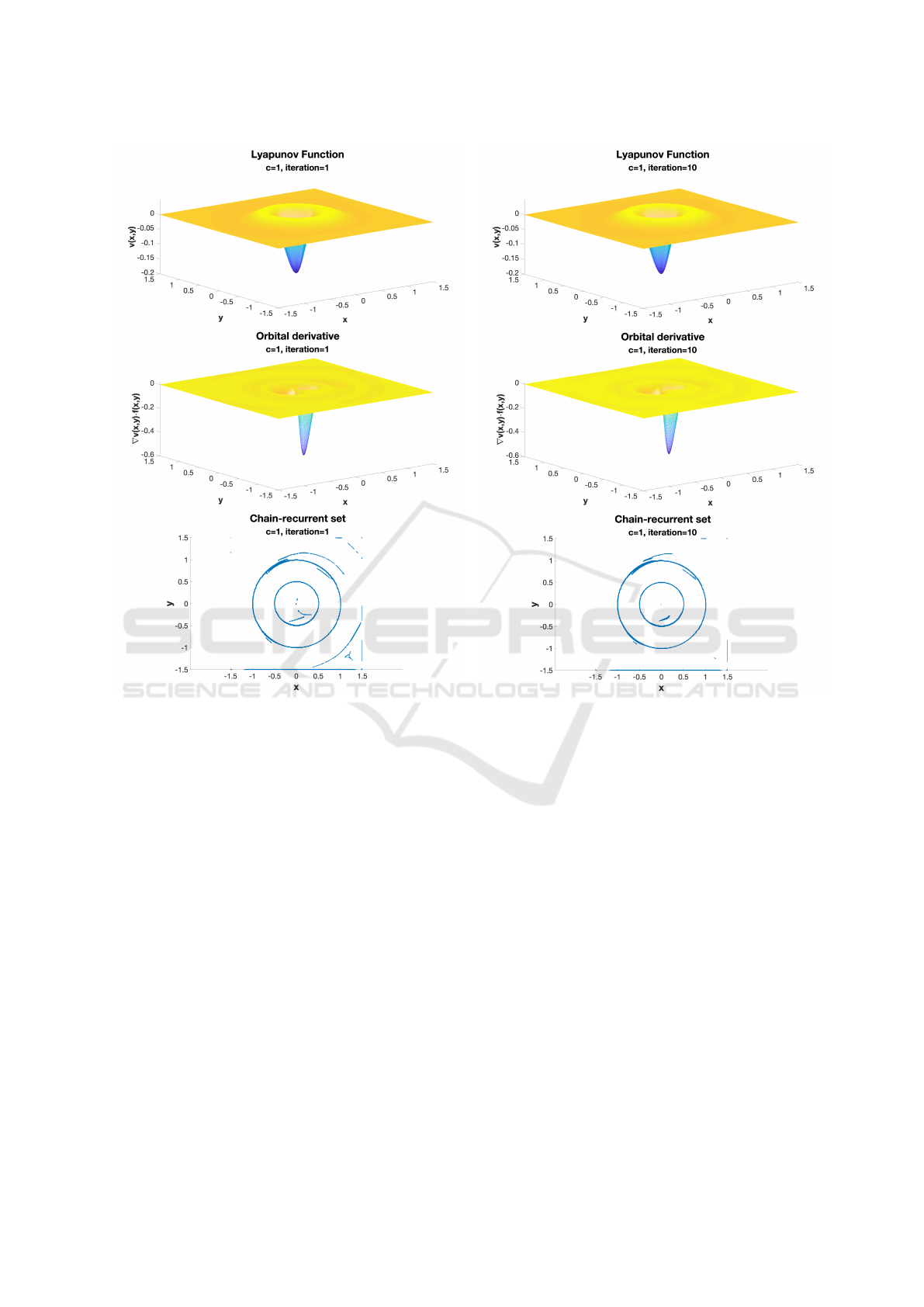
Figure 1: Above: Complete Lyapunov function. Middle:

Orbital derivative. Bottom: Chain-recurrent set. System

(18). First iteration, i.e., quadratic optimization. The nor-

malized method was used with c = 1 and δ

= 10

−8

3.2.2 Homoclinic Orbit

We consider system (1) with right-hand side f(x,y) =



x(1 − x

− y

) − y((x − 1)

+ (x

+ y

− 1)

)

y(1 − x

− y

) + x((x − 1)

+ (x

+ y

− 1)

)



(19)

This system has an unstable focus at the origin and

an asymptotically stable homoclinic orbit at a circle

centred at the origin and with radius 1.

The collocation points were set in (−1.5,1.5) ×

(−1.5,1.5) ⊂ R

with α

Hexa-basis

= 0.018, which gives

32,064 collocation points. An extra point, x

(0.1846,0) is added to fulﬁll the condition v

) =

−1 during the quadratic optimization.

Figure 2: Above: Complete Lyapunov function. Middle:

Orbital derivative. Bottom: Chain-recurrent set. System

(18). Tenth iteration, i.e., iterative method solving the PDE

to the values of the average values of the orbital derivatives

around the corresponding collocation points. The normal-

ized method was used with c = 1 and δ

= 10

−8

3.2.3 Van der Pol Oscillator System

We consider system (1) with right-hand side

f(x,y) =



(1 − x

)y − x



. (20)

System (20) is the two-dimensional form of the Van

der Pol oscillator. This describes the behaviour of

a non-conservative oscillator reacting to a non-linear

damping. The origin is an unstable focus, and the sys-

tem has an asymptotically stable periodic orbit.

The collocation points were set in (−4,4) ×

(−4,4) ⊂ R

with α

Hexa-basis

= 0.05, which gives

29,440 collocation points. An extra point, x

(0.1,0) is added to fulﬁll the condition V

) = −1

during the quadratic optimization.

Figure 5 shows the plots for v

and ﬁgure 6 shows

the plots for v

. Both ﬁgures used c = 1 for system

Evaluation of Lyapunov Function Candidates through Averaging Iterations

739

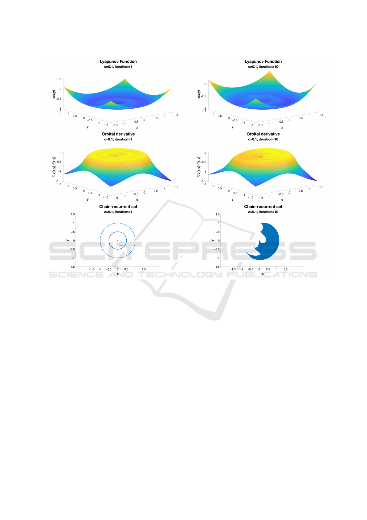
Figure 3: Above: Complete Lyapunov function. Middle:

Orbital derivative. Bottom: Chain-recurrent set. System

(18). First iteration, i.e., quadratic optimization. The nor-

malized method was used with c = 0.1 and δ

= 10

−8

(19). Likewise, ﬁgure 7 shows the plots for v

and

ﬁgure 8 shows the plots for v

. Both ﬁgures used

c = 0.1 for system (19).

Figure 9 shows the plots for v

and ﬁgure 10

shows the plots for v

. Both ﬁgures used c = 1 for

system (20). Likewise, ﬁgure 11 shows the plots for

and ﬁgure 12 shows the plots for v

. Both ﬁgures

used c = 0.1 for system (20).

3.3 Discussion of the Results

Let us discuss the results from our examples (18), (19)

and (20). Systems (19) and (20) do not show any im-

provement in the localization of the chain-recurrent

set when using iterations as seen in ﬁgures 5,6,7,8,9,

10, 11 and 12. System (18) shows slight improve-

ments, but only for c = 1. This clearly indicates that

the solution v

to the quadratic optimization prob-

lem (14) from (Giesl et al., 2018) cannot be improved

Figure 4: Above: Complete Lyapunov function. Middle:

Orbital derivative. Bottom: Chain-recurrent set. System

(18). Tenth iteration, i.e., iterative method solving the PDE

to the values of the average values of the orbital derivatives

around the corresponding collocation points. The normal-

ized method was used with c = 0.1 and δ

= 10

−8

by averaging iterations. We conclude that the norm-

minimization of the quadratic optimization problem

delivers a locally optimal solution, in the sense, that

averaging iterations do not improve the estimate of

the chain-recurrent set. Indeed, the estimates become

worse in most cases and, indeed, the approximation

form v

is quite good.

However, as solving the quadratic optimization

problem is much more computationally demanding

than solving a system of linear equations and iterat-

ing, one might try to obtain a solution v

using only

a few collocation points and then iterate on a denser

grid. We will investigate this in the future.

Even if in this paper we have presented all our re-

sults with the normalized method, it is very informa-

tive to have a look at the condition numbers of the

matrices involved in the examples, i.e. the matrix A

ICINCO 2020 - 17th International Conference on Informatics in Control, Automation and Robotics

740

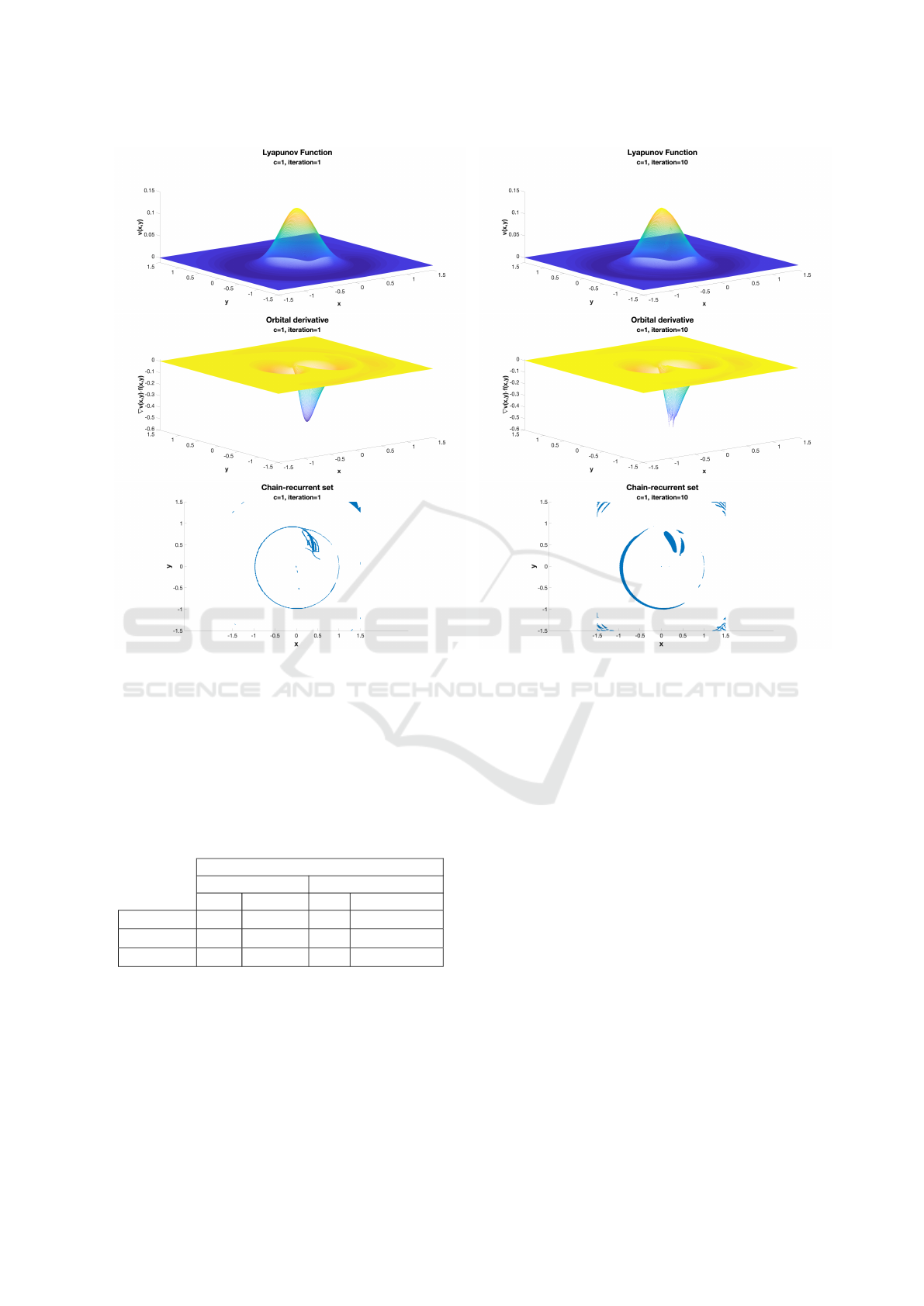
Figure 5: Above: Complete Lyapunov function. Middle:

Orbital derivative. Bottom: Chain-recurrent set. System

(19). First iteration, i.e., quadratic optimization. The nor-

malized method was used with c = 1 and δ

= 10

−8

from the collocation with and without the normalized

method.

Table 1: Condition number for the collocation matrices

computed for all systems under different values of c. Using

the system ODE directly on the left and normalized using

(17) on the right.

Condition number

Not normalized Normalized as (17)

c=1 c=0.1 c=1 c=0.1

ODE (18) 10

ODE (19) 10

ODE (20) 10

As it can be seen collocation matrices computed with

a Wendland function with support parameter c = 0.1

have much higher condition numbers, but this is to be

expected as there is more overlap of supports, the ma-

trix is less sparse, and the computed CLF candidate

is in general of much higher quality. The more inter-

esting observation is that using the normalization (17)

of the right-hand side of the ODE to obtain a system

Figure 6: Above: Complete Lyapunov function. Middle:

Orbital derivative. Bottom: Chain-recurrent set. System

(19). Tenth iteration, i.e., iterative method solving the PDE

to the values of the average values of the orbital derivatives

around the corresponding collocation points. The normal-

ized method was used with c = 1 and δ

= 10

−8

with a more uniform speed of traversing of trajecto-

ries delivers matrices with condition numbers that are

several orders of magnitude lower.

4 CONCLUSIONS

We investigated whether a complete Lyapunov func-

tion candidate computed by quadratic optimization

problem as in (Giesl et al., 2018) could be improved

by applying averaging iterations from (Arg

aez et al.,

2017; Arg

aez et al., 2018a; Arg

aez et al., 2018b;

Arg

aez et al., 2018c), which have been shown to de-

liver successively better approximations when start-

ing with an approximation to the ill-posed problem

(x) = −1. The result is that the complete Lyapunov

function candidate obtained by quadratic optimization

is locally optimal in the sense, that it cannot be im-

proved by these iterations.

Evaluation of Lyapunov Function Candidates through Averaging Iterations

741

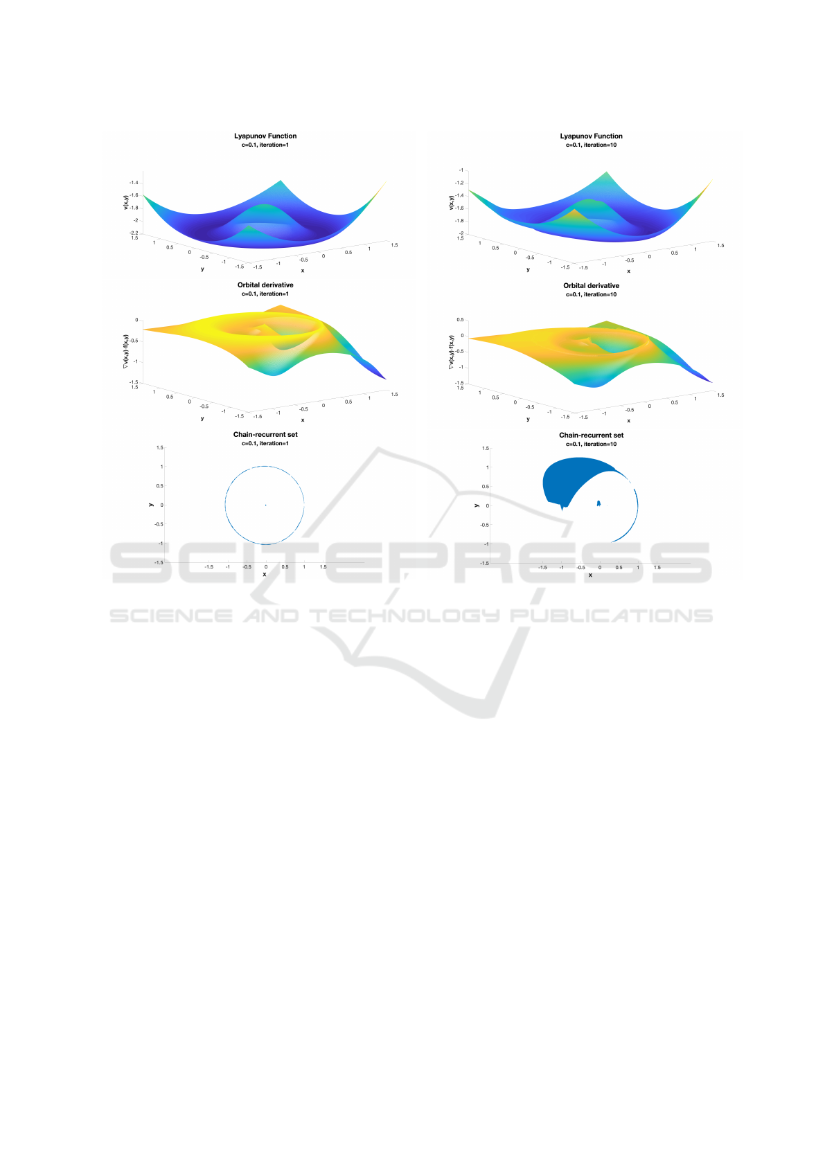
Figure 7: Above: Complete Lyapunov function. Middle:

Orbital derivative. Bottom: Chain-recurrent set. System

(19). First iteration, i.e., quadratic optimization. The nor-

malized method was used with c = 0.1 and δ

= 10

−8

ACKNOWLEDGEMENTS

The research in this paper is supported by the Ice-

landic Research Fund (Rann

ıs) grant number 163074-

052, Complete Lyapunov functions: Efﬁcient numer-

ical computation.

REFERENCES

Arg

aez, C., Giesl, P., and Hafstein, S. (2017). Analysing

dynamical systems towards computing complete Lya-

punov functions. In Proceedings of the 7th In-

ternational Conference on Simulation and Model-

ing Methodologies, Technologies and Applications,

Madrid, Spain, pages 323–330.

Arg

aez, C., Giesl, P., and Hafstein, S. (2018a). Com-

putation of complete Lyapunov functions for three-

dimensional systems. In Proceedings of the 57th IEEE

Conference on Decision and Control (CDC), pages

4059–4064, Miami Beach, FL, USA.

Figure 8: Above: Complete Lyapunov function. Middle:

Orbital derivative. Bottom: Chain-recurrent set. System

(19). Tenth iteration, i.e., iterative method solving the PDE

to the values of the average values of the orbital derivatives

around the corresponding collocation points. The normal-

ized method was used with c = 0.1 and δ

= 10

−8

Arg

aez, C., Giesl, P., and Hafstein, S. (2018b). Computa-

tional approach for complete Lyapunov functions. In

Awrejcewicz J. (eds) Dynamical Systems in Theoret-

ical Perspective. DSTA 2017., volume 248. Springer

Proceedings in Mathematics and Statistics. Springer,

Cham.

Arg

aez, C., Giesl, P., and Hafstein, S. (2018c). Iterative

construction of complete Lyapunov functions. In Pro-

ceedings of 8th International Conference on Simula-

tion and Modeling Methodologies, Technologies and

Applications - Volume 1: SIMULTECH,, pages 211–

222. INSTICC, SciTePress.

Ban, H. and Kalies, W. (2006). A computational approach

to Conley’s decomposition theorem. J. Comput. Non-

linear Dynam, 1(4):312–319.

Bernard, P. and Suhr, S. (2018). Lyapunov functions of

closed cone ﬁelds: from Conley theory to time func-

tions. Commun. Math. Phys., 359:467–498.

ornsson, J., Giesl, P., Hafstein, S., Kellett, C., and Li, H.

(2015). Computation of Lyapunov functions for sys-

tems with multiple attractors. Discrete Contin. Dyn.

Syst. Ser. A, 35(9):4019–4039.

ICINCO 2020 - 17th International Conference on Informatics in Control, Automation and Robotics

742

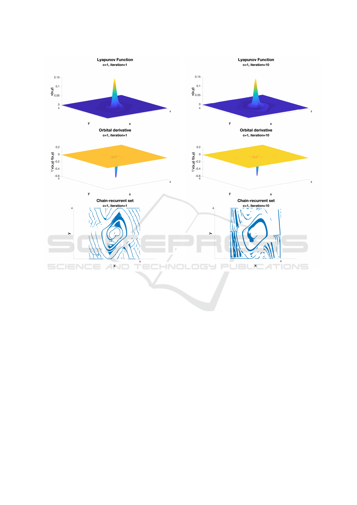
Figure 9: Above: Complete Lyapunov function. Middle:

Orbital derivative. Bottom: Chain-recurrent set. System

(20). First iteration, i.e., quadratic optimization. The nor-

malized method was used with c = 1 and δ

= 10

−8

Conley, C. (1978). Isolated Invariant Sets and the Morse

Index. CBMS Regional Conference Series no. 38.

American Mathematical Society.

Dellnitz, M., Froyland, G., and Junge, O. (2001). The algo-

rithms behind GAIO – set oriented numerical methods

for dynamical systems. In Ergodic theory, analysis,

and efﬁcient simulation of dynamical systems, pages

145–174, 805–807. Springer, Berlin.

Fathi, A. and Pageault, P. (2019). Smoothing Lyapunov

functions. Trans. Amer. Math. Soc., 371:1677–1700.

Giesl, P. (2007). Construction of Global Lyapunov Func-

tions Using Radial Basis Functions. Lecture Notes in

Math. 1904, Springer.

Giesl, P., Arg

aez, C., Hafstein, S., and Wendland, H. (2018).

Construction of a complete Lyapunov function using

quadratic programming. In Proceedings of the 15th

International Conference on Informatics in Control,

Automation and Robotics (ICINCO 2018), pages 560–

568.

Giesl, P. and Wendland, H. (2007). Meshless collocation:

Figure 10: Above: Complete Lyapunov function. Middle:

Orbital derivative. Bottom: Chain-recurrent set. System

(20). Tenth iteration, i.e., iterative method solving the PDE

to the values of the average values of the orbital derivatives

around the corresponding collocation points. The normal-

ized method was used with c = 1 and δ

= 10

−8

error estimates with application to Dynamical Sys-

tems. SIAM J. Numer. Anal., 45(4):1723–1741.

Goullet, A., Harker, S., Mischaikow, K., Kalies, W., and

Kasti, D. (2015). Efﬁcient computation of Lyapunov

functions for Morse decompositions. Discrete Contin.

Dyn. Syst., 20(8):2419–2451.

Hurley, M. (1992). Noncompact chain recurrence and at-

traction. Proc. Amer. Math. Soc., 115:1139–1148.

Hurley, M. (1998). Lyapunov functions and attractors

in arbitrary metric spaces. Proc. Amer. Math. Soc.,

126:245–256.

Iske, A. (1998). Perfect centre placement for radial ba-

sis function methods. Technical Report TUM-M9809,

TU Munich, Germany.

Kalies, W., Mischaikow, K., and VanderVorst, R. (2005).

An algorithmic approach to chain recurrence. Found.

Comput. Math, 5(4):409–449.

Narcowich, F. J., Ward, J. D., and Wendland, H. (2005).

Sobolev bounds on functions with scattered zeros,

Evaluation of Lyapunov Function Candidates through Averaging Iterations

743

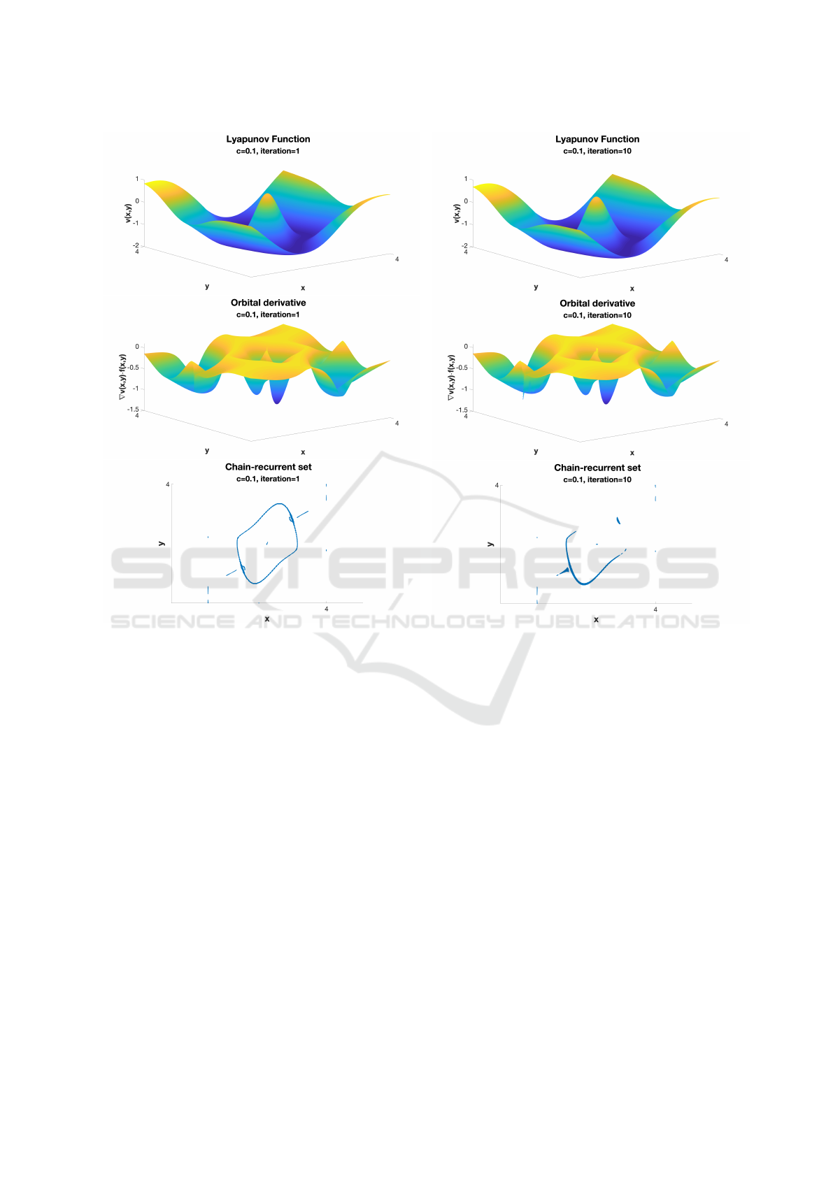
Figure 11: Above: Complete Lyapunov function. Middle:

Orbital derivative. Bottom: Chain-recurrent set. System

(20). First iteration, i.e., iterative method solving the PDE

to the values of the average values of the orbital derivatives

around the corresponding collocation points. The normal-

ized method was used with c = 0.1 and δ

= 10

−8

with applications to radial basis function surface ﬁt-

ting. Mathematics of Computation, 74:743–763.

Suhr, S. and Hafstein, S. (2020). Smooth complete Lya-

punov functions for ODEs. submitted.

Wendland, H. (1995). Piecewise polynomial, positive deﬁ-

nite and compactly supported radial functions of min-

imal degree. Adv. Comput. Math., 4(4):389–396.

Wendland, H. (1998). Error estimates for interpolation by

compactly supported Radial Basis Functions of mini-

mal degree. J. Approx. Theory, 93:258–272.

Wendland, H. (2005). Scattered data approximation, vol-

ume 17 of Cambridge Monographs on Applied and

Computational Mathematics. Cambridge University

Press, Cambridge.

Figure 12: Above: Complete Lyapunov function. Middle:

Orbital derivative. Bottom: Chain-recurrent set. System

(20). Tenth iteration, i.e., iterative method solving the PDE

to the values of the average values of the orbital derivatives

around the corresponding collocation points. The normal-

ized method was used with c = 0.1 and δ

= 10

−8

ICINCO 2020 - 17th International Conference on Informatics in Control, Automation and Robotics

744