
Automatic Ontology Learning from Domain-specific Short Unstructured
Text Data
Yiming Xu
1 a
, Dnyanesh Rajpathak
2 b
, Ian Gibbs
3 c
and Diego Klabjan
4 d
1
Department of Statistics, Northwestern University, Evanston, U.S.A.
2
Advanced Analytics Center of Excellence, Chief Data & Analytics Office, General Motors, U.S.A.
3
Customer Experience (CX) Organization, General Motors, U.S.A.
4
Department of Industrial Engineering and Management Sciences, Northwestern University, Evanston, U.S.A.
Keywords:
Ontology Learning, Information Systems, Classification, Clustering.
Abstract:
Ontology learning is a critical task in industry, which deals with identifying and extracting concepts reported in
text such that these concepts can be used in different tasks, e.g. information retrieval. The problem of ontology
learning is non-trivial due to several reasons with a limited amount of prior research work that automatically
learns a domain specific ontology from data. In our work, we propose a two-stage classification system
to automatically learn an ontology from unstructured text. In our model, the first-stage classifier classifies
candidate concepts into relevant and irrelevant concepts and then the second-stage classifier assigns specific
classes to the relevant concepts. The proposed system is deployed as a prototype in General Motors and its
performance is validated by using complaint and repair verbatim data collected from different data sources. On
average, our system shows the F1-score of 0.75, even when data distributions are vastly different.
1 INTRODUCTION
Over 90% of organizational memory is captured in the
form of unstructured as well as structured text. The
unstructured text takes different forms in different in-
dustries, e.g. body of email messages, warranty repair
verbatim, patient medical records, fault diagnosis re-
ports, speech-to-text snippets, call center data, design
and manufacturing data and social media data. Given
the ubiquitous nature of unstructured text it provides a
rich source of information to derive valuable business
knowledge. For example, in an automotive (which is
used as our running example) or aerospace industry in
the event of fault or failure, repair documents (com-
monly referred to as verbatim) are captured (Rajpathak
et al., 2011). These repair verbatims provide a valu-
able source of information to gain an insight into the
nature of fault, symptoms observed along with fault,
and corrective actions taken to fix the problem after
systematic root cause investigation (Rajpathak, 2013).
It is important to extract the knowledge from such ver-
a
https://orcid.org/0000-0003-3011-700X
b
https://orcid.org/0000-0002-1706-5308
c
https://orcid.org/0000-0003-0286-952X
d
https://orcid.org/0000-0003-4213-9281
batims to understand different ways by which the parts,
components, modules and systems fail during their us-
age and under different operating conditions. Such
knowledge can be used to improve the product quality
and more importantly to ensure an avoidance of similar
faults in the future. However, efficient and timely ex-
traction, acquisition and formalization of knowledge
from unstructured text poses several challenges: 1.
the overwhelming volume of unstructured text makes
it difficult to manually extract relevant concepts em-
bedded in the text, 2. the use of lean language and
vocabulary results into an inconsistent semantics, e.g.
‘vehicle’ vs ‘car,’ or ‘failing to work’ vs. ‘inopera-
tive,’ and finally, and 3. different types of noise are
observed, e.g. misspellings, run-on words, additional
white spaces and abbreviations.
An ontology (Gruber, 1993) provides an explicit
specification of concepts and resources associated with
domain under consideration. A typical ontology (or a
taxonomy) may consist of concepts and their attributes
commonly observed in a domain, relations between
the concepts, a hierarchical representation of concepts
and concept instances representing ground-level ob-
jects. For example, the concept ‘vehicle’ can be used
to formalize a locomotive object and vehicle instances,
Xu, Y., Rajpathak, D., Gibbs, I. and Klabjan, D.
Automatic Ontology Learning from Domain-specific Short Unstructured Text Data.
DOI: 10.5220/0009980100290039
In Proceedings of the 12th International Joint Conference on Knowledge Discovery, Knowledge Engineering and Knowledge Management (IC3K 2020) - Volume 3: KMIS, pages 29-39
ISBN: 978-989-758-474-9
Copyright
c
2020 by SCITEPRESS – Science and Technology Publications, Lda. All rights reserved
29

such as ‘Chevrolet Equinox.’ An ontological frame-
work and the concept instances can be used to share
the knowledge among different agents in a machine-
readable format (e.g. RDF/S
1
) and in an unambiguous
fashion. Hence, ontologies constitute a powerful way
to formalize the domain knowledge to support different
application, e.g. natural language processing (Cimiano
et al., 2005) (Girardi and Ibrahim, 1995), information
retrieval (Middleton et al., 2004), information filtering
(Shoval et al., 2008), among others.
Given the overwhelming scale of data in the real
world and an ever-changing competitive technology
landscape, it is impractical to construct an ontology
manually that scales at an industry level. To overcome
this limitation, we propose an approach whereby an
ontology is constructed by training a two-stage ma-
chine learning classification algorithm. The classifier
to extract and classify key concepts from text consists
of two stages: 1. in the first stage, a classifier is trained
to classify the multi-gram concepts in a verbatim into
relevant concepts and irrelevant concepts and 2. in the
second stage, the relevant concepts are further classi-
fied into their specific classes. It is important to note
that a concept can be a relevant in one verbatim, e.g.
‘check engine light
is on
,’ but irrelevant in another ver-
batim, e.g. ‘vehicle
is on
the driveway.’ Our input
text corpus consists of short verbatims and the goal is
to identify additional new concepts and classify them
into their most appropriate classes. In the first-stage,
our classifier takes as the input labelled training data
consisting of
n
-grams generated from each verbatim
and the label related to each
n
-gram, where
n
ranges
from 1 to 4. The labelling process is performed manu-
ally and also by using an existing incomplete domain
ontology. More specifically, if a concept is already
covered in a domain ontology then its existing class
is used as a label for a
n
-gram; otherwise a human
reader provides a label. In our classification model,
we use both linguistic features (e.g. part of speech
(POS)), positional features (e.g. start and end index in
verbatim, length of verbatim), and word embedding
features (word2vec (Mikolov et al., 2013)). The prob-
lem of polysemy poses a significant challenge since
they occur frequently in short text. In our approach,
we introduce a new feature that handles the problem
of polysemy as follows: Given a 1-gram, we cluster
their embedding vectors with the number of clusters
equal to the number of polysemy of a 1-gram based on
WordNet (Miller, 1995) and then for an occurrence of a
1-gram, we use centroid of the closest cluster as a rep-
resentative feature. For higher n-grams, e.g. 4-gram
we observe limited positive samples in the training
data and we perform two rounds of active learning to
1
https://www.w3.org/TR/rdf-schema/
boost the number of positive samples. Our two-stage
classification model is deployed as a proof-of-concept
in General Motors and the experiments have shown it
to be an effective approach to discover new concepts
of high quality.
Through our work, we claim the following key con-
tributions. 1. In real-world industry, data comes from
disparate sources and therefore, the relevant concepts
are heterogeneous both in terms of the lean language
(e.g. ‘unintended acceleration’ and ‘lurch forward’)
and distributions. We successfully identify collabora-
tive, common set of features to train a machine learn-
ing classification model that classifies heterogeneous
concepts with high accuracy. 2. The problem of poly-
semy, e.g. ‘car
on
driveway’ v.s. ‘check engine light
is
on
’ is ubiquitous in our data. A new type of feature
named polysemy centroid feature (discussed in section
4.3) is introduced, which handles the problem of pol-
ysemy in our data. 3. Abbreviations are common in
real-world data and their disambiguation is important
for the correct interpretation of data. We successfully
disambiguate abbreviations and to the best of knowl-
edge ours is the first proposal to disambiguate domain-
specific abbreviations by combining a statistical and a
machine learning model. 4. The proposed model is a
practical system that is deployed as a tool in General
Motors for an in-time augmentation of domain specific
ontology. The system is scalable in nature and handles
the industrial scale repair verbatim data.
The rest of the paper is organized as follows. In
the next section, we provide a review of the relevant
literature. In Section 3, the problem description and
an overview of our approach are discussed. In Section
4, we discuss data preprocessing algorithms that are
used to clean the data and then discuss the process of
feature engineering to identify key features that are
used to train the classifiers. In Section 5, we discuss
in detail the experiments and evaluation of our classi-
fication models. In Section 6, we conclude our paper
by reiterating the main contributions and giving future
research directions.
2 BACKGROUND AND RELATED
WORKS
A plethora of works have been done in ontology learn-
ing (Lehmann and Völker, 2014). There were three
major approaches: statistical methods (e.g. weirdness,
TF-IDF), machine learning methods (e.g. bagging,
Naïve Bayes, HMM, SVM), and linguistic approaches
(e.g. POS patterns, parsing, WordNet, discourage anal-
ysis).
(Wohlgenannt, 2015) built an ontology learning
KMIS 2020 - 12th International Conference on Knowledge Management and Information Systems
30

system by collecting evidence from heterogeneous
sources in a statistical approach. The candidate con-
cepts were extracted and organized in the ‘is-a’ rela-
tions by using chi-squared co-occurrence significance
score. In comparison with (Wohlgenannt, 2015), we
use a structured machine learning approach, which
can be applied on unseen datasets. In (Wohlgenannt,
2015), all evidence was integrated into a large seman-
tic network and the spreading activation method was
used to find most important candidate concepts. The
candidate concepts are then manually evaluated before
adding to an ontology. In comparison with this, in
our approach the latent features, e.g. context features,
polysemy features from the data are identified to train
a machine learning classifier. Hence, it exploits richer
data characteristics compared to (Wohlgenannt, 2015).
Finally, ours is a probability based classifier and it
can be applied to any new data to extract and classify
important concepts effectively. The only manual inter-
vention involved in our approach is to assign labels to
the
n
-grams included in the training data. Finally, the
model proposed by (Wohlgenannt, 2015) is determin-
istic in nature and it does not consider the notion of
context. Hence, it is very difficult to imagine how such
model can be generalized to extract concepts specified
in different context in the new data.
(Doing-Harris et al., 2015) makes use of the co-
sine similarity, TF-IDF, a C-value statistic, and POS
to extract the candidate concepts to construct an ontol-
ogy. This work was done in a statistical and linguistic
approach. The key difference between our work and
the one proposed in (Doing-Harris et al., 2015), is
ours is a principled machine learning model. It makes
our system scalable to extract and classify multi-gram
terms from industrial scale new data without manual
intervention. The linguistic features, e.g. POS exploits
syntactic information for better understanding text.
(Yosef et al., 2012) constructs a hierarchical on-
tology by employing support vector machine (SVM).
The SVM model heavily relies on the part-of-speech
(POS) as the primary feature to determine classifica-
tion hyperplane boundary. In comparison to (Yosef
et al., 2012), in our approach the POS is used as one of
the features, but we also consider additional features,
such as the context, polysemy, and word embedding to
establish the context of a unigram or multi-gram con-
cepts. Moreover, we also perform two rounds of active
learning to further boost the classifier performance. As
word embedding features are not considered by (Yosef
et al., 2012) it is difficult to envisage how the context
associated with each concept was considered during
their extraction.
(Pembeci, 2016) evaluates the effectiveness of
word2vec features in ontology construction. The statis-
tic based on 1-gram and 2-gram counts was used to
extract the candidate concepts. However, the actual
ontology was then constructed manually. In our work,
we not only train a word2vec model to develop word
embedding based context features, but other critical
features, such as POS, polysemy features, etc. are also
used to train a robust probabilistic machine learning
model. The word embedding features included in our
approach dominate statistical features and, therefore,
other statistical features are not used in our approach.
(Ahmad and Gillam, 2005) constructs an ontology
by using the ‘weirdness’ statistic. The collocation
analysis was performed along with domain expert ver-
ification process to construct a final ontology. There
are two key differences between our approach and the
one proposed by (Ahmad and Gillam, 2005). Firstly,
in our approach the labelled training data along with
different features as well as stop words are used to
train a classification model, while in their approach
the notions of ‘weirdness’ and ‘peakedness’ statistics
are used to extract the candidate concepts. Secondly,
in their work, there was a heavy reliance on domain
experts to verify and curate newly constructed ontol-
ogy. With our approach, no such manual intervention
is needed during concept extraction stage or classifi-
cation stage. Hence, our system can be deployed as a
standalone tool to learn an ontology from an unseen
data.
In our work, we also propose a new approach to
disambiguate abbreviations. There are several related
works. (Stevenson et al., 2009) extract features, such
as concept unique identifiers and then built a classifi-
cation model. (HaCohen-Kerner et al., 2008) identify
context based features to train a classifier, but they
assumed an ambiguous phrase only with one correct
expansion in the same article. (Li et al., 2015) pro-
pose a word embedding based approach to select the
expansion from all possible expansions with largest
embedding similarity. There are two major differences
between our approach and these works. First, we
propose a new model that seamlessly combines the
statistical approach (TF-IDF) with machine learning
model (Naïve Bayes classifier). That is, we measure
the importance of each concept in terms of TF-IDF
and then estimate the posterior probability of each
possible expansion. Alternate approaches either only
apply machine learning model or simply calculate sta-
tistical similarity between abbreviation and possible
expansions. Second, in these works a strong assump-
tion is made that each abbreviation only has a single
expansion in the same article and therefore the features
are conditionally independent. No such assumption is
made in our approach and therefore it is more robust.
Automatic Ontology Learning from Domain-specific Short Unstructured Text Data
31

3 PROBLEM STATEMENT AND
APPROACH
In industry, data comes from several disparate sources
and it can be useful in providing valuable information.
However, given the overwhelming size of real-world
data, manual ontology creation is impractical. More-
over, there are limited systems reported in literature
that can be readily tuned to construct an ontology from
the data related to different domains. In this work, we
primarily focus on unstructured short verbatim text
(commonly collected in automotive, aerospace, and
other heavy equipment manufacturing industries).
This is a typical verbatim collected in automotive
industry: "Customer states the engine control light is
illuminated on the dashboard. The dealer identified in-
ternal short to the fuel pump module relay and the fault
code P0230 is read from the CAN bus. The fuel pump
control module is replaced and reprogrammed. All the
fault codes are cleared." As shown in Figure 1, the
domain model (classes and relations among them) of
a specific domain, e.g. automotive, is designed by the
domain experts, which have the common understand-
ing of a domain. Our algorithm is trained by using a
training dataset from a specific domain. In the first
stage, the objective is to extract and classify all the rele-
vant technical concepts reported in each verbatim, such
as ‘engine control light’, ‘fuel pump module relay’, ‘is
illuminated’, ‘internal short’, ‘fuel pump control mod-
ule’, and ‘replaced and reprogrammed’. In the second
stage, the relevant concepts are further classified into
their specific classes. For instance,
part:
(engine con-
trol light, fuel pump module relay, fuel pump control
module),
symptom:
(is illuminated, internal short),
and
action:
(replaced and reprogrammed). The clas-
sified technical concepts populates the domain model,
which can be used within different applications, such
as natural language processing, information retrieval,
fault detection and root cause investigation, among
others.
The classification process in our approach starts by
constructing a corpus of millions of verbatims. Since a
corpus usually contains different types of noise, these
noises are cleaned by using a text cleaning pipeline.
It consists of misspelling correction, run-on words
correction, removal of additional white spaces, and ab-
breviation disambiguation. From each verbatim, all the
stop words are deleted due to their non-descriptive na-
ture and because they do not add any value to classifier
training by using the domain specific vocabulary. Next,
each verbatim is converted into
n
-grams (
n = 1, 2, 3, 4
)
and these
n
-grams constitute the training data. For
each
n
-gram, labels are assigned to indicate whether
it is a relevant technical or irrelevant non-technical
concept and also a specific class (e.g. part, symptom,
action in case of automotive domain) is assigned to
each relevant technical concept. The labelling task is
performed by using an existing seed ontology and also
by using human reviewers. The process of generating
the training dataset is discussed in further in Section
4.2.
As we discuss in Section 4.3, we identify several
unique features related to each
n
-grams, such as POS,
polysemy, word2vec, etc. The labeled
n
-grams and
their corresponding features are used to train our clas-
sification model. The relevant concepts and their fea-
tures are then fed to the second stage classification
model, which is trained to assign specific classes to
them. In our domain, the number of positive samples
decrease as the size of
n
-gram grows. Hence, the train-
ing data consists of a limited number of 4-grams. To
overcome this problem, two rounds of active learning
are performed to boost the number of training sam-
ples of 4-grams in the training data. Active learning
also helps to improve the overall performance of our
model. In the inference stage (i.e. when applied on
the new data), the model takes raw verbatims and pre-
processes by using our data cleaning pipeline and then
it extracts all candidate concepts without stop words
and noise words. Finally, these candidate concepts
are fed as input to our two-stage classification system.
Figure 2 shows the overall process of our two-stage
classification system.
4 MODEL SPECIFICATIONS
As discussed in the previous section, our data consists
of different types of noise and it is important to clean
the raw data before it can be used for feature engineer-
ing and then to train our classifiers. Below, we discuss
each data cleaning steps in further details.
4.1 Data Preprocessing
In particular, four different data cleaning algorithms
are used to clean the data: misspelling correction,
run-on words correction, removal of additional white
spaces, and abbreviation disambiguation.
1. Misspellings Correction.
We consider all possible
corrections of a misspelled 1-gram each with Leven-
shtein distance of 1. If there is only one correction,
we replace the misspelled 1-gram by the correction.
Otherwise, for each candidate correction we define
its semantic similarity score to be the product of its
logarithm of frequency and the word2vec similarity
between the misspelled 1-gram and its correction. The
KMIS 2020 - 12th International Conference on Knowledge Management and Information Systems
32
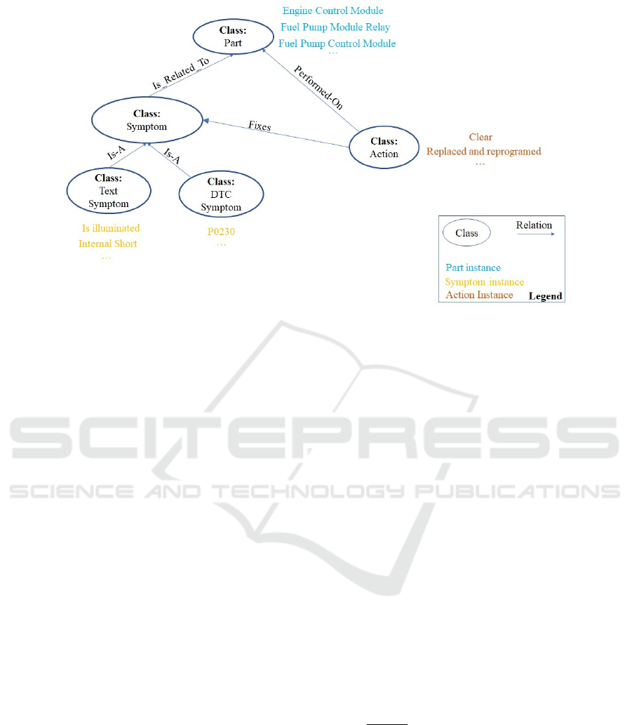
Figure 1: The domain model is designed by the domain experts. The classifier is trained to extract the technical concepts and
they are classified into their specific classes to populate the domain model.
misspelled 1-gram is replaced by the correction with
the maximum similarity score.
2. Run-on Words Correction.
We split run-on words
into a 2-gram by inserting a white space between each
pair of neighboring characters. For a specific split, if
both the left 1-gram and the right 1-gram are correct we
retain such split as the correct one. If there are multiple
possible splits with correct 1-grams, then for each
correct split its semantic similarity score is defined to
be the maximum of word2vec similarities between the
run-on 1-gram and the two 1-grams. The split with
maximum similarity score is replaced as the correct
split.
3. Removal of Additional White Spaces.
We also
observe several cases in the data where there are ad-
ditional white spaces inserted in a 1-gram, e.g. ‘actu
ator.’ We try to remove the additional white spaces
to see whether it turns the two incorrect 1-grams into
a correct 1-gram and if it does, then we employ this
correction.
4. Abbreviation Disambiguation.
The use of abbre-
viations, e.g. ‘TPS is shorted’ is ubiquitous in a corpus
and it is critical to disambiguate their meaning to cor-
rectly populate our domain model. Typically, an abbre-
viation is a concept that can be mapped to more than
one possible expansion (or full form), for example,
‘TPS’ could stand for ‘Tank Pressure Sensor,’ ‘Tire
Pressure Sensor’ or ‘Throttle Position Sensor.’ The
abbreviations mentioned in our data are identified by
using the domain specific dictionary, which consists of
commonly observed abbreviations and their possible
full forms. For an identified abbreviation with a single
full form, we replace that specific abbreviation with its
full form. Otherwise we employ the following model.
Suppose an abbreviation
abbr
(e.g. TPS) has
N
possible full forms, namely,
{ f f
1
, f f
2
, ..., f f
N
}
,
where
N > 1
. For ‘TPS’ we have three possible full
forms: ‘Tank Pressure Sensor,’ ‘Tire Pressure Sen-
sor’ or ‘Throttle Position Sensor.’ We first collect
the 1-gram concepts, which co-occur with
abbr
from
the entire corpus. The context concepts co-occurring
with
abbr
are denoted as
C
abbr
and the set of all co-
occurring concepts related to each possible expansion,
say
f f
n
,
1 ≤ n ≤ N
are denoted as
C
n
. To prevent
meaningless expansions and to compare the posterior
probabilities of
f f
i
and
f f
j
, we only focus on the in-
tersection of these sets:
V = ∩
N
n=1
C
n
∩C
abbr
. Having
identified the relevant intersecting context concepts,
we measure the importance of each concept that is a
member of intersection in terms of its TF-IDF score.
Let
v
u
∈ R
|V|
be the TF-IDF vector of collocate
u = abbr
or full form
u = f f
i
. Given that
f f
n
is asso-
ciated with
abbr
, the probability of co-occurring con-
cepts given
f f
n
is then estimated as
P(abbr| f f
n
) =
∏
|V|
i=1
(
v
f f
n
,i
|V |
∑
j=1
v
f f
n
, j
)
v
abbr,i
.
This formula computes a probability and if
abbr
and
f f
n
are truly interchangeable then they have
the same underlying distribution probability of their
co-occurring concepts. Furthermore, we estimate
the prior probability
P( f f
n
)
of
f f
n
from its docu-
ment frequency. Therefore, by the Bayes theorem,
P( f f
n
|abbr) ∝ P(abbr| f f
n
) ·P( f f
n
)
. We then replace
abbreviation
abbr
by the full form with the largest
Automatic Ontology Learning from Domain-specific Short Unstructured Text Data
33
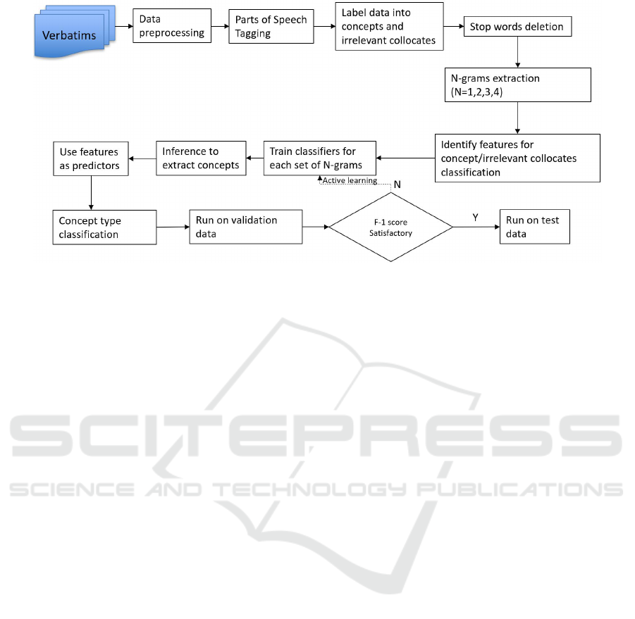
Figure 2: The overall methodology and flow of the two-stage classification model.
posterior probability.
4.2 Preparation of Training Set
The process of classifying the data starts by labeling
the raw
n
-grams generated from the cleaned data to
construct the training set. Given the scale of real-world
data, it is impossible to manually label each raw sam-
ple. To overcome this problem, we make use of the
seed (incomplete) ontology and tag all such n-grams
that are already covered in the seed ontology with the
label. For instance, if a specific
n
-gram, e.g. ‘engine
control light’ is already covered in the existing seed
ontology then it is assigned the label of relevant tech-
nical concept and then a specific class of a ‘n’-gram
is borrowed from the seed ontology, e.g. the technical
concept ‘engine control light’ is assigned a specific
class ‘part.’ For the purpose of avoiding repetitions
and keeping concepts as complete as possible, only
the longest concepts are marked as a true concept.
That is, in a specific verbatim a concept ‘engine con-
trol module’ is marked as the relevant concept, then
its sub-grams, such as ‘engine’, ’control’, ‘module’,
’engine control’, ’control module’ are labelled as irrel-
evant concepts in that specific verbatim. Since the seed
ontology is incomplete it is difficult to imagine that it
covers all the
n
-grams included in the training dataset.
The
n
-grams that are not covered in the seed ontology
are labelled by domain experts. Please note that we
impose a specific frequency threshold (tuned empiri-
cally) and the
n
-grams with their frequency above the
threshold are used for manual labelling.
In inference, given a verbatim, we collect all pos-
sible
n
-grams without stop words and noise words in
them and they are passed to the two-stage classification
system.
4.3 Feature Engineering
In our model, different types of features, such
as discrete linguistic features, word2vec features,
polysemy centroid features, and the context based
features are identified.
1. Discrete Linguistic Features.
From the data the
following linguistic features are identified: 1) the POS
tags related to each
n
-gram is used which is assigned
by employing Stanford parts of speech tagger (Ratna-
parkhi, 1996), 2) the POS tags of the three nearest left
side 1-grams of the
n
-gram, 3) the POS tags of the
three nearest right side 1-grams of the
n
-gram, 4) the
POS tag of the nearest concept on the left side of the
n
-gram, 5) the POS tag of the nearest concept on the
right side of the n-gram.
2. Word2vec Features.
We also consider the continu-
ous word2vec vector associated with each
n
-gram as
one of the features to improve the model performance.
We train a Skip-Gram model with respect to frequent
1-grams. When the word2vec embedding is not avail-
able, we consider it as a zero vector. For a
n
-gram,
the associated feature vector is the average word2vec
embedding of all its 1-grams.
3. Context Features.
We consider the ‘context’
word2vec feature of each
n
-gram. For a
n
-gram
T
, we
take the 3 left 1-grams and 3 right 1-grams of
T
in the
verbatim and then obtain the word2vec embeddings of
6 1-grams. The context feature is constructed by the
concatenation of the average of the 3 embeddings on
the left and the average of the 3 embeddings on the
right. If a specific
n
-gram is towards the beginning
or an end of a verbatim and then naturally less than 3
embeddings get constructed, but in such cases all the
empty
n
-grams are not considered while constructing
KMIS 2020 - 12th International Conference on Knowledge Management and Information Systems
34

the average embedding. If none of the context terms
are available (in our domain it is possible that only one
n
-gram makes a complete sentence), we set an average
embedding to be the zero vector.
4. Polysemy Centroid Features.
In our data, the
n
-grams appearing in different verbatim may have dif-
ferent semantic meanings as their context changes.
Given the number of meanings of a specific
n
-gram
extracted from WordNet, we cluster all the context
features of such
n
-gram into a specific number of clus-
ters. We take a viewpoint that the cluster centroid of
each cluster essentially provides a representative fea-
ture (indicative of different meanings) of a
n
-gram. In
this way, we distinguish between different semantic
meanings of the same
n
-gram based on its context.
Specifically, we consider the polysemy of a 1-grams
and the following two steps as shown in Figure 3 are
employed: 1. For each
n
-gram
T
, we randomly sample
1,000 verbatims in which
T
is mentioned and calculate
the context feature vector
V (T)
for
T
in each selected
verbatim. Then, we use WordNet to obtain the number
p
polysemies of
T
. Further, the k-Means clustering
algorithm is used to cluster these 1,000
V (T)
vectors,
with the number of clusters set to
p
. 2. Having gener-
ated polysemy centroids for a
n
-gram
T
0
, we find the
context vector from its verbatim. The feature vector
of
T
0
corresponds to the closest centroid among those
obtained in step 1 for
T
0
with respect to the context
features of T
0
.
Figure 3: (1) Obtain all possible polysemy centroids of a col-
locate: for a collocate
T
, we cluster context vectors and save
the cluster centroids
C
1
(T ), ...,C
p
(T )
. (2) Create polysemy
centroid feature of a collocate: for a new collocate
T
0
, let
m = argmin{d(V(T
0
),C
1
(T
0
)), ..., d(V(T
0
),C
p
0
(T
0
))}
de-
note the index of the closest centroid, where
d
is the Eu-
clidean distance. Vector
C
m
(T
0
)
is our polysemy feature for
T
0
.
5. Features based on the Incomplete Ontology. We
also find that a seed ontology plays a significant role
in classification. For a n-gram, we split it into 1-grams
and add a feature vector of the same length as the
n
-gram, with each element being set to be 1 if such
1-gram exists in the seed ontology, otherwise 0.
4.4 Classification
In our work, we train a random forest model as our clas-
sification model, but we have also experimented with
support vector machine, gradient boosted trees, and
Naïve Bayes models. The model selection experiments
showed that the random forest model outperformed all
other models. As a part of model training process, we
fine-tune the following important hyperparameters of
random forest: the number of trees in the forest is 10,
no maximum depth of a tree, the minimum number of
samples required to split an internal node is 2.
To further boost model performance, we have also
introduced two rounds of active learning. For this,
eight different classifiers are trained by feeding ran-
domly sampled data. All the samples with four positive
and four negative votes are collected. We then pass all
such samples that the classifiers fail to classify consis-
tently into their correct classes to human reviewers for
manual labelling. All the samples generated from the
two rounds of active learning are added to the training
data.
We also analyze feature importance by using the
backward elimination process. Within the backward
elimination process, our model initially starts with
all features and then randomly drops one feature at a
time, and we train a new model by using the remain-
ing features. This is done for all features. Then we
remove the feature that yields the largest improvement
to the F1-score when removed. This process is re-
peated iteratively until removing any feature does not
improve the F1-score. The final set of features kept
are Word2vec, Polysemy, POS, Context and Existing
Ontology, which are the most important features in our
model. The features dropped are left POS, right POS,
left three POSes, right three POSes.
5 COMPUTATIONAL STUDY
In this section, we provide experimental results to val-
idate our model. While our model can be applied
to any domain, in our work, we validate our ontol-
ogy learning system on a subset of an automotive
repair (AR) verbatim corpus collected from an auto-
motive original equipment manufacturer, the vehicle
ownership questionnaire (VOQ) complaint verbatim
collected from National Highway Traffic Safety Ad-
ministration
2
, and Survey data. The AR data contains
more than 15 million verbatims, each of which on
average contains 19 1-grams. Here is a typical AR
verbatim: "c/s service airbag light on. pulled codes
P0100 & ..solder 8 terminals on both front seats as per
special policy 300b.clear codes test ok." The classifica-
tion models are trained on AR. To study the generality
of our model, we also test on VOQ, which contains
2
https://www.nhtsa.gov/
Automatic Ontology Learning from Domain-specific Short Unstructured Text Data
35

more than 300,000 verbatims. The VOQ verbatims are
significantly different from AR primarily because the
VOQ verbatim are reported directly by customers, and
thus they are more verbose and less technical in nature
in comparison with AR. A sample from VOQ reads:
"heard a pop. all of the sudden the car started rolling
forward...." Finally, the Survey data is generated from
the telephone conversation between customer and ser-
vice representative. It also consists of different faults
as the ones reported in AR, but they are longer with
more description. Our existing seed ontology consists
of about 9,000
n
-grams associated with three different
classes, labeled as Part, Symptom, and Action herein.
The classification system is implemented in Python
2.7 and Apache Spark 1.6 and ran on a 32-core Hadoop
cluster. The extracted ontology is added to the cen-
tral database where it can be accessed by different
business divisions, e.g. service, quality, engineering,
manufacturing. Below we discuss the evaluation of the
abbreviation disambiguation as well as both the stages
of our classification model.
5.1 Evaluation of Abbreviation
Disambiguation
To evaluate the performance of the abbreviation dis-
ambiguation algorithm, we generate three separate test
datasets from the AR data source. On average, 5%
of AR verbatims contain an abbreviation and each
abbreviation has more than 2 expansions. Table 1 sum-
marizes the results of the abbreviation disambiguation
algorithm experiment. All the results are manually
evaluated by domain experts.
Table 1: The result summary of abbreviation disambiguation
algorithm.
N
raw
denotes the number of raw verbatims,
N
c
denotes the number of abbreviations corrected and
N
correct
denotes the number of correct abbreviation corrections.
Data N
raw
N
c
N
correct
Accuracy
AR 1 10,000 204 154 0.75
AR 2 30,000 374 278 0.74
AR 3 45,000 407 312 0.77
As it can be seen in Table 1, the performance of
the algorithm is stable, i.e. accuracy does not vary
across the three test datasets. On average, 75% of our
corrections are correct, which shows our algorithm is
able to capture correct expansions of abbreviations.
Note that there might be abbreviations that are not
captured by our algorithm if abbreviations are not in
the abbreviation list.
5.2 Performance of Classifiers
One of the bottlenecks of supervised machine learning
approach is to assemble a large volume of manually
labeled data. Recall that the training data is from the
AR data. Since the entire AR data is large, our training
set is sampled from AR in the following way: for each
n
-gram (
n = 1, 2, 3, 4
), we randomly sample 50,000
relevant and irrelevant concepts, which we regard as
the training set for the
n
-gram model. Among 100,000
training samples, only 2,000
n
-grams are manually
labeled and 2,000 are generated by active learning. For
evaluation, we generate three different test datasets.
The datasets are first preprocessed using the data
preprocessing pipeline (cf. Section 4.1) and the
cleaned data are used in inference. The first test dataset
consists of 3,000 randomly selected repair verbatim
from the AR data. The model classified
n
-grams into
relevant and irrelevant concepts and then classified
the relevant concepts into their specific classes of ei-
ther Part, Symptom, or Action. We then randomly
selected 1,500 classified
n
-grams for their evaluation
by domain experts to calculate precision, recall and
F1-score. The second test dataset consists of 23,000
VOQ verbatims and from the classified
n
-grams we
randomly selected 1,500
n
-grams for their evaluation
by domain experts. The third test dataset consists of
46,000 verbatims and from the classified
n
-grams we
randomly selected 1,000
n
-grams for their evaluation
by domain experts. The randomly drawn samples used
in evaluation are reviewed in the context of actual ver-
batim in which they are reported. Moreover, in the AR
test set among those
n
-grams classified as the relevant
concepts, slightly less than 30% of concepts are newly
discovered by our algorithm, which are not previously
covered in the seed ontology. This is a useful finding
because newly discovered concepts provide additional
coverage to detect new faults/failures for improved
decision making. Please also note that the proposed
system is not evaluated against other algorithms that
are presented in the related work, because the systems
reported in the literature are end-to-end solutions and
to make a fair comparison all the components used
by these systems are necessary. The precision, recall,
and F1-score for the test datasets based on the domain
expert results are given in Table 2.
Table 2: The evaluation of relevant concepts and irrelevant
concepts classification algorithm.
Dataset Precision Recall F1-score
AR 0.81 0.90 0.85
VOQ 0.89 0.47 0.62
Survey 0.80 0.79 0.79
KMIS 2020 - 12th International Conference on Knowledge Management and Information Systems
36

As we can observe in Table 2, the classification
F1-score on the AR dataset of relevant and irrelevant
concepts is relatively high since the test and training
sets are from the similar distribution, in which case
the ontology learning system performs very well. In
VOQ, since the test data is not from a similar distri-
bution, i.e. the VOQ verbatims are more verbose, the
performance on VOQ data is much worse than that on
AR. The Survey data is conditionally sampled from
AR, and therefore is also from a similar distribution
as training, which results in good classification per-
formance. Moreover, on AR, the F1-score for each
n
-gram is 0.88, 0.81, 0.83, 0.86 for
n = 1, 2, 3, 4
, re-
spectively. The F1-score for 1-gram is better primarily
because we have a polysemy centroid feature to cap-
ture polysemy meanings of 1-grams, which very likely
have different polysemies. For higher grams, the per-
formance is also good, and we presume this is because
longer concepts are more easily captured by the algo-
rithm while shorter concepts can be easily confused
with irrelevant n-grams.
Table 3: The evaluation of relevant concept type classifica-
tion algorithm.
Dataset Precision Recall F1-score
AR 0.82 0.82 0.82
VOQ 0.84 0.65 0.73
Survey 0.82 0.80 0.81
We follow the same approach to evaluate the perfor-
mance of the second stage classifier which takes as the
input the relevant concepts classified by the first stage
classifier and assigns specific classes, i.e. Part, Symp-
tom, or Action. The test set sizes are 800, 1,500, 900
for AR, VOQ and Survey respectively. Note that the
‘concepts’ passed to the second stage classifier could
be incorrectly classified by the first stage classifier,
i.e. some inputs could be irrelevant concepts. Each
irrelevant concept input to the second stage classifier
is counted as falsely predicted regardless of the type
predicted by the classifier. Despite of this, as it can
be seen from Table 3, the second stage classification
model shows good precision rate, but the recall rate
is comparatively lower, due to the false negative rate,
i.e. the classifier misses out on assigning types to long
phrases. It is important to note that although the VOQ
dataset is generated from a completely different data
source, the second stage classifier shows a very good
performance.
Next, we calculate feature importance by record-
ing how much F1-score drops when we remove each
feature. The higher the value, the more important the
feature. As it can be seen in Figure 4, the features that
contribute most to the F1-score are Word2Vec, Con-
Figure 4: Change of F1-score when dropping each feature.
text, Polysemy and POS, which is consistent with our
observation in backward elimination algorithm. The
two most important features are Polysemy (4.3%) and
Word2vec (3.8%), which shows the significance of
applying word embeddings to the problem of ontology
learning.
Table 4: Examples of classification results, where ‘None’
denotes irrelevant concepts.
Collocate Predicted True Type
RECOVER Action Action
NO POWER PUSHED None None
HIGH MOUNT BRAKE BULB Part Part
PARK LAMP None Part
ROUGH IDLE RIGHT SIDE Part None
ENGINE CUTS OFF None Symptom
Table 4 shows typical examples of the correctly
and incorrectly classified relevant and irrelevant con-
cepts. There are some critical reasons that are iden-
tified which contribute to the misclassification. First,
the POS tags associated with each concept considered
during the training stage is one of the crucial features
and it turns out that POS tags assigned by the Stan-
ford’s POS tagger are inconsistent in our data. For
example, in ‘PARK LAMP,’ the POS tagger tags it
as ‘VBN NNP,’ while it should be tagged as ‘NNP
NNP’ since ’PARK’ here is not a verb. Second, there
is variance in stop and noise words in real-world data.
While standard English stop words and noise words
allow us to reduce the non-descriptive concepts in the
data, we need a more comprehensive stop and noise
word customized dictionary specific to automotive do-
main. Moreover, such a dictionary needs to be a living
document that requires timely augmentation to ensure
as complete coverage to such words as possible. For
example, ‘OFF,’ which is usually regarded as a stop
word in English should not be in our customized stop
words list as it appears in concepts like ‘ENGINE
CUTS OFF.’ Third, concepts that are combinations of
two different class types contribute to misclassification.
In our data, concepts such as ‘ENGINE CUTS OFF’
Automatic Ontology Learning from Domain-specific Short Unstructured Text Data
37

consist of two classes fused together, i.e. ‘ENGINE’
is class Part, while ‘CUTS OFF’ is class Symptom. To
handle such cases, we need to have more representa-
tives within the training dataset.
We also perform another experiment in order to
assess the effectiveness of our model in re-discovering
the relevant concepts that are already included in the
existing seed ontology. For this experiment, we ran-
domly removed the relevant concepts related to the
three classes, referred to as class Part, class Symp-
tom, and class Action in the existing seed ontology.
Specifically, we removed 250 class Part concepts, 127
class Symptom concepts, and 23 class Action concepts.
Since the concepts in the seed ontology are acquired
from the AR data, 12,000 AR verbatim are used in
this experiment. The test dataset of 12,000 verbatim is
cleaned and the trained classification model is applied.
The model extracted and classified the relevant and
irrelevant concepts and then the relevant concepts are
classified into Part, Symptom or Action. Table 5 shows
the results of this experiment in terms of precision, re-
call, and F1-score.
Table 5: The reconstruction of existing seed ontology from
the AR data.
Technical class Precision Recall F1-score
Part 0.89 0.83 0.85
Symptom 0.86 0.79 0.82
Action 0.90 0.86 0.88
As it can be seen from Table 5, our classification
model has shown promising F1-score and identified
the key relevant concepts that were randomly removed
from the seed ontology. The closer analysis of the
results revealed that our model suffered particularly
in classifying 4-grams concepts. There are two rea-
sons behind this: 1. In some cases, the correction of
4-gram concepts by the data cleaning pipeline showed
limited accuracy. For example, a 4-gram concept ‘P S
STEERING RACK’ was converted into ‘Power Steer-
ing Steering Rack’ (as the first two 1-grams ‘P’ and ‘S’
are converted into ‘Power’ and ‘Steering’). Then clas-
sifier marked such concept as a member of class Part,
but a domain expert considers it to be an irrelevant
concept. 2. As discussed earlier, the Stanford POS
tagger assigns inconsistent tags to the class Symptom
concepts in our domain. Further investigation revealed
that the Stanford POS tagger assigns a POS tag to
a term by estimating a tag sequence probability, i.e.
p(t
1
. . . t
n
|w
1
. . . w
n
) =
∏
n
i=1
p(t
i
|t
1
. . . t
i−1
, w
1
. . . w
n
) ≈
∏
n
i=1
p(t
i
|h
i
).
In our domain, this notion of maximum likelihood
showed weaknesses primarily due to the sparse context
words associated with higher
n
-grams. Since the con-
text words around 4-grams change based on verbatim
in which they appear the same concept gets different
POS tags. For example, the concept ‘air pressure com-
pressor sensor’ in one verbatim gets the POS tag of
‘NNP NN NN NN,’ while in another verbatim it is
tagged as ‘NN NN NN NN.’ The POS is one of the
important features in our classification model, which
ends up impacting the classification accuracy. There-
fore, it is important to note that our model shows good
F1-score given the complex nature of real-world data,
both in terms of identifying new concepts as well as in
reconstructing existing concepts.
The ontology learning system discussed in this
work is deployed in General Motors. The proposed
model is run once every two months in order to extract
and classify new concepts, which are reported in the
AR data. The newly extracted concepts are added
to the existing ontology to improve in-time coverage.
This new ontology provides a semantic backbone to
the ‘fault detection tool,’ which is used to build the
fault signatures from different data sources to identify
key areas of improvement.
6 CONCLUSION
We propose an effective and efficient two-stage classi-
fication system for automatically learning an ontology
from unstructured text. The proposed framework ini-
tially cleans noisy data by correcting different types
of noise observed in verbatims. The corrected text
is used to train our two-stage classifier. In the first
stage, the classification algorithm automatically clas-
sifies
n
-grams into relevant concepts and irrelevant
concepts. Next, the relevant concepts are classified
to their specific classes. In our approach, different
types of features are used and we not only use surface
features, e.g. POS, but also identify latent features,
such as word embeddings and polysemy features as-
sociated with
n
-grams. In particular, the introduction
of novel polysemy controid feature helps in correctly
classifying
n
-grams. As shown in the evaluation, the
combination of surface features together with latent
features provides necessary discrimination to correctly
classify collocates. The evaluation of our system using
real-world test data shows its ability to extract and clas-
sify
n
-grams with high F1-score. The proposed model
has been successfully deployed as a proof of concept
in General Motors for an in-time augmentation of a
domain ontology.
In the future, our aim is to extend our model to
handle
n
-grams with their length greater than 4 and
also intend to develop a deep learning approach to
further improve the performance of our system.
KMIS 2020 - 12th International Conference on Knowledge Management and Information Systems
38

REFERENCES
Ahmad, K. and Gillam, L. (2005). On the move to mean-
ingful internet systems 2005: Coopis, doa, and odbase.
pages 1330–1346.
Cimiano, P., Hotho, A., and Staab, S. (2005). Learning
concept hierarchies from text corpora using formal
concept analysis. Journal of Artificial Intelligence
Research, 24(1):305–339.
Doing-Harris, K., Livnat, Y., and Meystre, S. (2015). Au-
tomated concept and relationship extraction for the
semi-automated ontology management (seam) system.
Journal of Biomedical Semantics, 6(1):15.
Girardi, M. and Ibrahim, B. (1995). Using English to retrieve
software. Journal of Systems and Software, 30(3):249–
270.
Gruber, T. R. (1993). A translation approach to portable
ontology specifications. Knowledge Acquisition,
5(2):199–220.
HaCohen-Kerner, Y., Kass, A., and Peretz, A. (2008). Com-
bined one sense disambiguation of abbreviations. Pro-
ceedings of the 46th Annual Meeting of the Association
for Computational Linguistics on Human Language
Technologies: Short Papers, pages 61–64.
Lehmann, J. and Völker, J. (2014). Perspectives on ontology
learning. In Studies on the Semantic Web. IOS Press.
Li, C., Ji, L., and Yan, J. (2015). Acronym disambiguation
using word embedding. Association for the Advance-
ment of Artificial Intelligence Conference.
Middleton, S. E., Shadbolt, N. R., and De Roure, D. C.
(2004). Ontological user profiling in recommender
systems. ACM Transactions on Information Systems,
22(1):54–88.
Mikolov, T., Chen, K., Corrado, G., and Dean, J. (2013).
Efficient estimation of word representations in vector
space. CoRR, abs/1301.3781.
Miller, G. A. (1995). Wordnet: A lexical database for En-
glish. Communications of the ACM, 38(11):39–41.
Pembeci, I. (2016). Using word embeddings for ontology en-
richment. International Journal of Intelligent Systems
and Applications in Engineering, 4(3):49–56.
Rajpathak, D. G. (2013). An ontology based text mining
system for knowledge discovery from the diagnosis
data in the automotive domain. Computers in Industry,
64(5):565–580.
Rajpathak, D. G., Chougule, R., and Bandyopadhyay, P.
(2011). A domain-specific decision support system for
knowledge discovery using association and text mining.
Knowledge and Information Systems, 31:405–432.
Ratnaparkhi, A. (1996). A maximum entropy model for
part-of-speech tagging. Empirical Methods in Natural
Language Processing.
Shoval, P., Maidel, V., and Shapira, B. (2008). An ontology-
content-based filtering method. International Journal
of Theories and Applications, 15:303–314.
Stevenson, M., Guo, Y., Al Amri, A., and Gaizauskas, R.
(2009). Disambiguation of biomedical abbreviations.
Proceedings of the Workshop on Current Trends in
Biomedical Natural Language Processing, pages 71–
79.
Wohlgenannt, G. (2015). Leveraging and balancing het-
erogeneous sources of evidence in ontology learning.
The Semantic Web. Latest Advances and New Domains,
pages 54–68.
Yosef, M. A., Bauer, S., Hoffart, J., Spaniol, M., and
Weikum, G. (2012). Hyena: Hierarchical type classifi-
cation for entity names. 24th International Conference
on Computational Linguistics, pages 1361–1370.
Automatic Ontology Learning from Domain-specific Short Unstructured Text Data
39
