Overview on Modeling for Control of Autonomous Road Vehicles Platoon

Nacer K. M’Sirdi

1 a

, Abdelhak Dahmani

and Habib Nasser

2,†

Aix Marseille University, Universit

e de Toulon, CNRS, LIS UMR 7020, SASV, Marseille, France

RDI’UP (Innovative Research), 2 Rue Louis Bl

eriot, 78130 Les Mureaux, France

†

https://www.rdiup.com/

Keywords:

Vehicles Fleet, Fleet Modeling, Modelling and Control Approach.

Abstract:

This is an overview on the models used to control ﬂeets of road vehicles. In general, simpliﬁed vehicle models

are used and their coupling features are introduced through the (individual) controllers. The robustness and

precision of motion control needs geometric, kinematic and dynamic descriptions. We propose a modeling

methodology for robots platooning to introduce speciﬁc features in the platoon behavior. This overview pro-

poses reference models to link the ﬂeet vehicles and assign a character to the group independent from control.

1 INTRODUCTION

1.1 Context and Objectives

To increase the capacity of the infrastructures while

improving the safety and the comfort, vehicle pla-

tooning is of interest. Several solutions are consid-

ered, in the urban environment and on the highway,

by automating vehicles driving and autonomous ﬂeet

control (Nouveliere et al., 2002; Alcala et al., 2018;

Allou and Zennir, 2018). This can be a very efﬁcient

means of transportation for passengers and freight and

for increasing trafﬁc capacity. For example, a convoy

of trucks carries goods, with only one driver (Bauer

and Tomizuka, 1996; M’Sirdi, 2018). Other beneﬁts,

such as reducing fuel consumption and minimizing la-

bor, may exist in piggybacking or truck-mounted cars.

The convoy consists of a leading vehicle and trailing

trucks. The leader can be autonomous or manually

driven, other vehicles follow him with a safety dis-

tance to avoid collisions between vehicles.

Depending on the application purpose, a lot of ve-

hicle models have been considered in the literature

(Nouveliere et al., 2002; Alcala et al., 2018; Allou

and Zennir, 2018). The representation is, in general,

simpliﬁed and the ﬂeet control is at a level higher than

the one of the embedded feedback (local level of the

DoF or actuators). Robust control laws, can avoid the

use of precise models, but this means that all efforts

are done in control (Menhour et al., 2015).

https://orcid.org/0000-0002-9485-6429

The nonlinear robust control approaches give the

ﬂeet a better controlled and more robust behavior

against uncertainties (Szanto et al., 2020; Lenain,

2005; Guillet et al., 2014). In this type of ap-

proach, the disadvantages are the availability of in-

formation on the vehicles of the chain, the need for

sensors, the communication of the data, and the ob-

servability. There is still a lack of inter vehicles rela-

tions,environment interactions and global strategy.

There is no general modelling methodology. The

main focus of this paper is the ﬂeet modeling and in-

formation contained in the models. It is well known

that there exists also robust control approaches, avoid-

ing models or considering only integrators in the pro-

cess (Menhour et al., 2015). Indeed, the entire vehicle

dynamic controllability must be mobilized to perform

safe driving and emergency maneuvers like an obsta-

cle or slipping avoidance and urgent controlled brak-

ing (Ali et al., 2015; M’Sirdi, 2018). The models used

for ﬂeets control focus on the representation of rela-

tive trajectories of the vehicles. Some of them con-

sider only longitudinal motion (1D) and few of them

are 2D. Each modeling approach suggests or more ap-

propriate control approaches (M’Sirdi, 2020).

The organization of this paper is as follows. Af-

ter this introduction, the section 2 presents the convoy

models used in ﬂeets control. This is followed by a

general overview of the most often used control archi-

tectures (local and global). In section 3, inspired from

the nature, we propose a new modeling approach to

represent a ﬂeet of vehicles. This will allow to assign

a special character to the group and application of sev-

208

M’Sirdi, N., Dahmani, A. and Nasser, H.

Overview on Modeling for Control of Autonomous Road Vehicles Platoon.

DOI: 10.5220/0009971302080216

In Proceedings of the 17th International Conference on Informatics in Control, Automation and Robotics (ICINCO 2020), pages 208-216

ISBN: 978-989-758-442-8

 2020 by SCITEPRESS – Science and Technology Publications, Lda. All r ights reserved

eral non linear control approaches for the autonomous

ﬂeet driving. Then we conclude and give some per-

spectives on our work on observation and control of

robots platooning.

2 CONVOY MODELS USED IN

CONTROL

Table 1: Table of state variables and Acronyms.

L distance between the vehicle axles

The gravity center of vehicle i

distance from the front axle to G

distance from the rear axle to G

mass of vehicle i plus 2 wheels

Longitudinal position of vehicle i in R

Lateral position of vehicle i in R

Angular position of vehicle i in R

Orientation at M of ref Trajectory in R

Longitudinal vehicle position in R

Lateral vehicle position in R

Front Steering angle (input vehicle i)

rear Steering angle (d

= 0 in general)

i,i−1

longit distance inter vehicles i and i-1

i, j

lateral distance between vehicles i and j

input of the vehicle i

i, j

desired distance between vehicles

IVD: Inter Vehicles Distance

h IVSD Inter Vehicle Safety Distance

Curvilinear abcissa of the vehicle i

LDI Londitudinal Double Integrator

LUM Longitudinal Unidirectional Model

LBM Longitudinal Bidirectional Model

ACM Anti-Collision Margin

L distance between the vehicle axles

The gravity center of vehicle i

distance from the front axle to G

distance from the rear axle to G

c(s) Curvature tangent to Γ at M

Damping and Stifness of RM-IVDR

f , r, l, d Indices for front, rear, left and right sides

RM- Reference Model

IVDR Inter Vehicles Dynamic Relations

2.1 Longitudinal Control Models (1D)

In general, a set of simpliﬁed and individual 1D mod-

els are considered. The only interest of 1D models is

the study of the IVSD (Inter-Vehicle Safety Distance).

This type of model and its controls ignore the lateral

movement and curvatures of the trajectory. Note that

there is no relation between the vehicles equations ex-

cept by the relative distance variables e

, which is used

in the control only.

2.1.1 Longitudinal Unidirectional Models

(LUM)

The most used model, for the longitudinal control of

the convoy is the double Integrator (Swaroop, 1994).

The input u

is the force applied to the vehicle i.

¨x

= u

(1)

For the Longitudinal Unidirectional Model, some au-

thors add a mass and a damper (Avanzini, 2010). m

is the vehicle mass and b a damper. Many parameters

are neglected. The vehicles are considered indepen-

dent and linked only by the control.

m ¨x

+ b ˙x + k(x − d

) = u

(2)

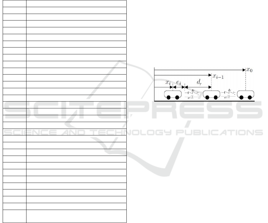
The desired relative Inter-Vehicle Distance IVD (see

ﬁgure 1) d

is considered in the control with the error

or relative distance to the preceding vehicle e

i,i−1

i, j

= x

− x

− (i − j)d (3)

Figure 1: LDI and LUM Mass-Spring-Damper.

2.1.2 Longitudinal Bidirectional Models (LBM)

The LBM is a second-order system and the distances

to the neighbors (preceding e

i,i−1

and following e

i,i+1

)

are fed back through the control (Avanzini, 2010). In

this scheme, the individual vehicle models are cou-

pled with the control interaction forces. Figure 1

shows a bidirectional longitudinal (mass, spring and

damper) model which link each vehicle to its neigh-

bors (previous and follower one).

2.1.3 LBM-VISD with Inter Vehicles Safety

Distance (IVSD)

The model dynamic equations, for a ﬂeet of n vehi-

cles, may be written as follows:











m ¨x

= k(x

− x

− d

1,2

) − c(˙x

− ˙x

) − h ˙x

+ u

m ¨x

= k(x

i−1

− x

− d

i−1,i

) − k(x

− x

i+1

− d

i,i+1

+c( ˙x

i−1

− 2 ˙x

+ ˙x

i+1

) − h ˙x

+ u

. . . . . .

m ¨x

= k(x

n−1

− x

− d

n−1,n

) − c(˙x

n−1

− ˙x

) − h ˙x

+ u

(4)

where k is the coefﬁcient of stiffness, c the damping

coefﬁcient and d the length of the spring (inter-vehicle

distance). The leading vehicle is driven by force input

control u

. It receives the forces of constraints trans-

mitted by the links springs - dampers, on the chain of

Overview on Modeling for Control of Autonomous Road Vehicles Platoon

209

the vehicles of the convoy. The inputs u

,...u

(not

used in the literature) may be zero or some comple-

mentary control inputs that we have added to enhance

the controllability.

• with either d

i−1,i

= d = constant and h = 0 ∀i.

This imposes an IVD. To ensure the stability of

the ﬂeet, according to the authors (Yanakiev and

Kanellakopoulos, 1996) (Avanzini, 2010), the ra-

tio c

/km must be greater than constants that in-

crease proportionally to the vehicle index i in the

convoy.

• or d

i−1,i

chosen for each vehicle i and h = 0 ∀i.

Another IVD has been proposed, to improve the

stability (Contet et al., 2009). It consists of choos-

ing, for each vehicle, a distance command d

i−1,i

between the vehicles of the convoy, according to

the state of the ﬂeet and stability constraints

• or d

i−1,i

= d = constant and h 6= 0. The Anti-

Collision Margin (ACM) h is added as a time dis-

tance margin to avoid collisions between vehicles

(Mu’azu et al., 2017).

The study of stability in (Contet et al., 2009), shows

that the bidirectional control architecture gives good

theoretical results when the number of vehicles of the

convoy is limited. In general, these models are used

for convoys that move at low speeds, do not take into

account the risk of failures, or the effects of errors

and noise measurement (Avanzini, 2010). Adding a

dynamics in the model has beneﬁts.

2.2 2D Convoy Models for Control

2.2.1 Unicycle Model (UCM)

A unicycle uses a minimal kinematic representation.

is the linear velocity of the vehicle i and ψ

is the

orientation angle of the vehicle wheel i (Samson and

Ait-Abderrahim, 1990; Xiang and Braunl, 2010; Ri-

cardo et al., 2008).







= v

.cos(ψ

)

= v

sin(ψ

)

= w

(5)

A study of chain transformation for a convoy is pro-

posed, to determine the Inter-Vehicle Distances (d

)

and the relative caps (γ) between the neighboring ve-

hicles. The control applied to the convoy vehicles is

based on a tangential linearization; The overall stabil-

ity has been proven for the linearized model.

2.2.2 Use of the Kinematic Models (KM)

Several applications use only a kinematic model, in a

2D space with limited speeds in the urban frame.

This is not advisable for a truck convoy

on the highway. Using a bidirectional con-

trol can alleviate the problem (Avanzini et al.,

2010). The model equations are presented

in equation (6). One can see a demo of this

model in open loop, by M Compere, in https:

//ch.mathworks.com/matlabcentral/ﬁleexchange/

67034-simple-animation-for-n-vehicles?focused=

9173618&tab=function











= v

.cos(ψ

) −

.sin ψ

= v

.sin(ψ

) +

.cos ψ

.δ

(6)

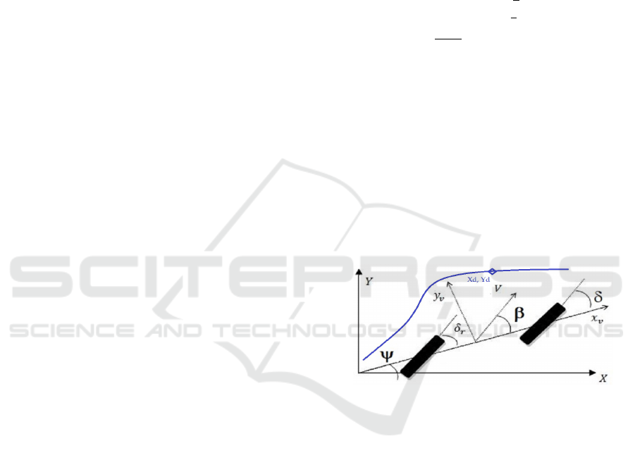
2.2.3 Kinematics Bicycle Model (KBM)

Geometric Convoy Model. Now we need to local-

ize the vehicle with regard to the reference trajectory

to be followed. The road reference path is noted Γ.

Figure 2 shows the geometric scheme of the vehicles

with regard to the path Γ in the absolute frame R

The vehicle is modeled with respect to the reference

path Γ (Lenain, 2005; Cartade et al., 2005). The ge-

ometric model deﬁnes the relations between vehicle

variables (in the vehicle frame R

) to Cartesian ones

and to the reference trajectory.

Figure 2: Bicycle Model.

Let us recall that ψ

is the orientation in the ab-

solute reference R

and l

denotes the desired IVSD

distance between 2 vehicles. Let s

be the curvilinear

abscissa of the vehicle i. This abscissa is at a distance

from the reference (desired) trajectory Γ (at point

M).

c(s): the curvature of the trajectory Γ at the point M

(s): Orientation of the tangent at M, in the absolute

frame R

(desired vehicle orientation)

= ψ

−ψ

(s) is the angular deviation of the vehicle

i relative to Γ.

= s

i−1

− s

− l

is the curvilinear spacing error, or

difference between 2 vehicles with a kinematic model

expressed as follows (see ﬁg 2).



X = v.cos(ψ

+ β)

Y = v.sin(ψ

+ β)

(7)

β denotes the side slip Angle

and δ

are the front and rear steering

ICINCO 2020 - 17th International Conference on Informatics in Control, Automation and Robotics

210

= Ψ

+ β is the vehicle motion angle







β = tan

−1

(

.tan(δ)+l

.tan(δ

)

Ψ =

v.cos(β)

.(tan(δ) − tan(δ

)

(8)

Assuming that δ

= 0 and β = 0, the Kinematics of

the system can be written as in equation (6)

Now, to be able to follow a trajectory (Γ) let us

deﬁne the desired position (Fig2) for the vehicle as

). We get ψ

= tan

−1

(

−Y )

− X)

) (9)

For the control, that there are two control inputs

(steering and velocity), we then deﬁne the curvilinear

trajectory errors (for the distance and the angle):



− X)

+ (Y

−Y )

= ψ

− ψ

(10)

For the longitudinal and lateral control (in Carte-

sian space R

) of a train of two vehicles following a

leader, in (Allou and Zennir, 2018), the authors use

multi-PID controllers (Optimized by PSO and Fuzzy

Logic) to compute the orientation and velocity of the

vehicle:

= PID(e

) = (K

+ K

.s)e

= PID(e

) = (K

+ K

.s)e

(11)

The two PID control parameters (K

) are optimized

by Particle Swarm (PSO) technique and by a fuzzy

approach. The parameter optimization is based on

a ﬁtness weight function Time Square Error (ITSE).

The drawback of this approach is the lack of dynam-

ics and that precise measurements of the absolute po-

sition variables is needed.

2.2.4 Dynamics Bicycle Model (DBM)

Also known as the Ackermann model, the DBM is

a Longitudinal and lateral model describing dynamic

and kinematic vehicle motions (Martinez et al., 2004;

Sprinkle et al., 2008). Its formulation varies from

one author to others (Daviet and Parent, 1996; Khatir

and Davidson, 2005; Bascetta et al., 2016; Zin et al.,

2004; Song et al., 2017; Huang et al., 2016).

DBM Decentralized Control. The simpliﬁed dy-

namic model (as presented in (Khatir and Davison,

2004)) is written in a three DoF system where v

de-

note the linear velocity of the vehicle i and θ

its wheel

orientation angle and β

the vehicle’s steering angle i.







m ˙v

= f

cos(β)

+ f

sin(β

)

= −

sin(β

) +

cosβ

− ψ

(12)

The bicycle Kinematics model is:







= v

cos(θ

+ β

)

= v

sin(θ

+ β

)

= ψ

(13)

Platoon of Autonomous Buses. In (Stanley and

Katupitiya, 2013b; Stanley and Katupitiya, 2013a),

the authors use the DBM with a different formulation

for each bus of a platoon dynamics. Their work is fo-

cused on the multi-agent systems to demonstrate the

ability for platoons to cooperatively maneuver around

each other. The kinematic equations are the same as

in eq 6:



= v

cosψ −

cosψ

= v

sinψ +

sinψ

(14)

with r=L/2 is the distance between the effective center

of rotation in the vehicle and the deﬁnite origin of the

vehicle, ψ as the vehicle orientation in a reference co-

ordinate system, and ω = ˙y as the vehicle body turning

rate. The dynamic equations, for each vehicle, are







X −

ψ) = R

− sinδF

− cosδ(T

− R

) − T

Y +

ψ) = − cos δ.F

+ F

+ sinδ.(T

− R

)

ψ = −l

.cos δ.F

+ l

.sin δ.(T

− R

)

(15)

T represents traction or propulsion, R the rolling re-

sistance and F the lateral forces on the wheels. The

slip angles are shown as the β

2.2.5 Robotics Models

The longitudinal and lateral positions and orientation

(X,Y,θ) of each vehicle i (with mass m

and inertia I

)

of the convoy are represented in a Cartesian frame R

is the gravity center of the vehicle, (v

) are its

longitudinal and lateral velocities.

Robotic Models are composed of Dynamic equa-

tions (eq 16, Kinematic transformation (see equation

6, and a geometric representation. This is why they

are more precise and advisable.

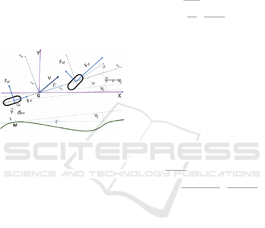
Dynamic Equations. The Lagrange method leads

to a set of dynamic equations (2.2.5) to describe the

motion of one vehicle (see the left scheme of ﬁgure

3), in the vehicle reference frame R

= (G

)

(Rabhi, 2005; DeSantis, 1995; Chebly, 2017). δ

the steering front wheel angle and ψ: the yaw angle.

The input force is F

= F

mot

and F

res

gathers

the resistance forces from the slope gravity and aero-

dynamics. The rolling resistance is ρ

and the road

slope is ζ.

res

= mg sin ζ +

ρAC

˙v

sgn( ˙v

) − ρ

Overview on Modeling for Control of Autonomous Road Vehicles Platoon

211

The longitudinal and lateral wheel forces are noted

x f

y f

. They can be got either trough the

wheel-road contact modeling or considering simply

longitudinal and lateral cornering stiffness for each

wheel (Rabhi, 2005) ( I

= I

+ 2I

+ m

+ l

)).

. ˙v

= F

x f

.cosδ

− F

y f

.sinδ

+ F

− F

res

. ˙v

+ a.m

ψ = F

x f

.sinδ

+ F

y f

.cosδ

+ F

+ a.m

˙v

= l

x f

sinδ

+ F

y f

cosδ

− F

y f

) − F

(16)

and l

are distances to G

from the front wheel and

from the rear wheel (respectively); a = l

− l

Figure 3: Bicycle Model and trajectory Γ.

The actuation dynamics when considered can be

written as follows, where J

are the wheels in-

ertia, rays, and motor torques. For a rear traction ve-

hicle T

= 0 and T

6= 0.



f i

= (T

− r

f i

x f

)

= (T

− r

)

(17)

Let us recall that the process has only 2 inputs (the

torque and the steering).

Geometric Model. The ﬁgure 3 shows the geomet-

ric scheme of the vehicles with the reference path γ in

the absolute frame R(0xy).

Let us note s

, the curvilinear abscissa (position

M) of vehicle i. The abscissa s

is located with respect

to a desired trajectory or trajectory Γ and we note d

the Side linear deviation of the vehicle i with respect

to the desired trajectory Γ.

is the center of the rear axle of the ith vehicle and

is the distance traveled (curvilinear abscissa) by the

closest point to O

on the path Γ. c(s

) is the curvature

of the Γ path in s

Recall that d

is the desired curvilinear distance be-

tween vehicles and c(S) is the curvature of the tra-

jectory C at the point M. The Curvilinear spacing be-

tween 2 vehicles is then: e

= s

i−1

− s

− d

= ψ−ψ

is the angular deviation of the vehicle

i relative to reference trajectory Γ.

The Kinematic equations are needed to get the

Curvilinear velocities ( ˙s

) to follow the motion of the

vehicle i and determine its orientation. The curvilin-

ear kinematic model can be written:











˙s

cos(

)

1− ˜y

.c(s)

˜y

= sin(

).v

= (

tanδ

−

c(s)cos(

)

1− ˜y

.c(s)

(18)

The kinematic modeling of vehicles, describes the

velocities based on the geometry of these vehicles.

The kinematic model alone does not completely rep-

resent the physical reality (Cordesses, 2000). The half

vehicle model, known as the bicycle, is an acceptable

representation for the dynamics of the convoy and is

most often used (Nadji, 2007; Nouveliere et al., 2002;

Lenain, 2005; Cartade et al., 2005).

These equations represent a non-holonomic sys-

tem, the state vector has three dimensions and two

dimensional control. The mathematical singularity

(s) = 1) will never appear because the point O

not at the center of the curve of the desired trajectory.

is the center of the rear axle of the ith vehicle. c(s

)

is the curvature of the Γ path in s

(Cordesses, 2000)

(see ﬁgures 3).

Some authors, to be complete, add to this model a

representation of wheel slip and drift angles (Lenain,

2005; Cartade et al., 2005; Petrov, 2009). If we con-

sider β

and β

the drift angles (front and back) of

the robot. The kinematics becomes then











˙s

= v

cos(

+β

)

1−c(s

) ˜y

˜y

= v

sin(

+ β

)

= cos(β

)

tan(δ

+β

)−tan(β

)

−

c(s

)cos(

+β

)

1−c(s

) ˜y

(19)

2.2.6 Conclusion on Vehicles Models

We have presented the models used for the control of

vehicle ﬂeets ranging from the simplest to the most

complete one. Several architectures have been used,

but there is still a lack of clear strategies non depen-

dent of the control laws used. For control of the vehi-

cle chain, the robotics models are the most appropri-

ate for the good motion control of the vehicles while

taking into account their dynamics and kinematic re-

lations. They involve correctly the transformations

from the vehicles operational variables to the Carte-

sian space representation.

Note that up to now, only the individual model of

one vehicle of the ﬂeet are considered and there is no

criteria on the global behaviour or the ﬂeet shape.

In section 3, we will propose a more complete

model, by adding to the robotics equations, a clear

description of the links and couplings of the vehicles

within the ﬂeet and with their environment.

ICINCO 2020 - 17th International Conference on Informatics in Control, Automation and Robotics

212

2.3 Control Architectures for Fleets

The existing control architectures can be classiﬁed

into several categories: Kinematic / Dynamic, Local /

Global, Uni or Bi-directional. This is related to the in-

formation used to control each vehicle. They are local

or global depending on sensor information they use to

control (Global: from all the vehicles, or Local only

neighbors). The two approaches can be unidirectional

(preceding neighbors) or bidirectional (neighbors in

front and behind).

2.3.1 Global Fleet Control Architecture

For the global or centralized architecture (GUC,

GBC), the control law applied to each vehicle of the

ﬂeet is based on the data (positions, velocities, ...) of

all the vehicles of the convoy (Yazbeck, 2014). Some-

times it can be partial, with data limited to the leader

and some of the neighboring vehicles, if the con-

voy chain is too long. For example, in partial GBC,

one uses the states variables of the leader and the 4

(front and rear plus left and right if any) or only 2

neighboring vehicles. This approach has been used

in (Caicedo et al., 2003), for a convoy moving in a

straight line. This makes global approaches more ex-

pensive(Ali et al., 2015).

2.3.2 Local or Decentralized Control

Architecture

In general, the most of vehicle pilots use only the in-

formation of the previous vehicle and possibly (only

partially) that of the following one (LUC, LBC). This

decentralized control (LUC) approach requires fewer

sensors and and very little information exchange be-

tween vehicles of the convoy, than the centralized ap-

proach. It also requires less computations and infor-

mation. The control is based on the data restricted to

neighbours in the convoy, to minimize the numbers of

the sensors used. (Qian et al., 2016; Nouveliere et al.,

2002; Sheikholeslam and Desoer, 1993).

2.3.3 Local Bidirectional Control Architecture

(LBC)

In bidirectional architecture, we are interested in in-

formation about the two neighbors,the previous vehi-

cle and the follower one. Each vehicle is controlled

targeting the previous one with regard to its followers

and leaders.

In this case, the disadvantages are the availability

of information on the vehicles of the chain, the need

for sensors, the communication of the data, and the

observability.

2.3.4 Local Unidirectional Control (LUC)

Each vehicle is controlled targeting the previous one

regardless to its follower. The driven vehicle in LUC

is slaved to follow its predecessor (Avanzini et al.,

2010). Tracking errors, introduced by sensors, actu-

ators, and delays accumulate from the leader vehicle

to the last one, in the convoy chain and affect the sta-

bility of the convoy motion. This causes oscillations

due to accumulated errors (Ali et al., 2015). This also

causes unacceptable disturbances if the string is long

(Avanzini, 2010). These problems are only partially

avoided in the global architecture.

3 NEW MODELING APPROACH

PROPOSED FOR PLATOONING

The robotic modeling approach seems more suitable

for driving ﬂeets of vehicles, robots or mobile de-

vices. Let us ﬁrst, discuss some observations of the

nature groups and then, we will use a more complete

architecture with a strategy that will consider models

including the group characteristics which is inspired

by the behavior of animals.

3.1 Modeling for Platooning

Two examples of ﬂeets of 5 vehicles will be used to il-

lustrate our modeling approach. They are represented

in ﬁgure (4). We will deﬁne the geometric model of

each vehicle and for the global ﬂeet. Using the ﬁve

gravity centers of the 5 vehicles we will deﬁne the

geometric form of the ﬂeet. Then, each vehicle is lo-

calized regard to the gravity center or the red vehicle

chosen as being the leader. Therefore the kinemat-

ics and ﬁnally the dynamic equations for each vehicle

will be considered.

Geometric Models in R

. If the red vehicle is the

leader of the ﬂeet 1 of the ﬁgure 4, its position is q

,ψ

]

, the preceding vehicle is at q

= q

[d,0,0]

the rear one at q

= q

+ [−d,0,0]

, the left

one at q

= q

+ [0,d

,0]

and the right one at q

+ [0,−d

,0]

, where d and d

are the longitudinal

and lateral IVSD. The geometric transformationis

kin





cosψ

−sin ψ

sinψ

cosψ

0 0 1





(20)

Kinematics Models. The Kinematic transforma-

tion matrix, for each vehicle, is the same as previously

Overview on Modeling for Control of Autonomous Road Vehicles Platoon

213

given (eq 6). We then get here:

= T

kin

. ˙q

= T

kin

. ˙q

= T

kin

. ˙q

= T

kin

. ˙q

= T

kin

. ˙q

Dynamic Models. The Lagrange method can be

used to get the (Inverse or Direct) Dynamic Model

equations, in the vehicle frame R

, (M’Sirdi et al.,

2007) for each vehicle, knowing it is related to its

neighbours (by τ

InverseDM U

= M

). ¨q

+ H

( ˙q

)

DirectDM ¨q

= M

)

−1

(−H

( ˙q

) +U

)

where U

= u

− τ

i+1

− τ

i−1

− τ

...

(21)

with the operational variables q

= [x

,ψ

]

the position vector for vehicle i, and ˙q

, ¨q

the velocity

and acceleration vectors. To this model we can add

the actuators (equation 17) and wheel ground contact

models (ignored here for the sake of simplicity and

considered in another control step).

Inter Vehicles Dynamic Relations (IVDR)

We introduce here the IVDR as a Reference Model

to include the constraints deﬁning the vehicles inter-

action dynamics (instead of only an intervehicle dis-

tance (constant or not); (τ

i−1

,τ

i+1

) are rear and front

constraints and (τ

,τ

) are from the left and right ve-

hicles in the ﬂeet 1 of the ﬁgure (4). We can have four

Reference Models (RM) for one vehicle and more RM

if we need. We can also relate all the vehicles to the

leader. We can also share a percentage of leading.

The forces τ

, represents the constraints (attrac-

tion/repulsion) from the nearby vehicles (front, rear,

left and right). This is the description of the relation

of the vehicle i to the other ones in the group (or pla-

toon). As an example, the relation with the preceding

vehicle could be, with a simple mass-spring-damper

model (for simplicity):

i+1

= M

. ¨e

i,i+1

+ B

i. ¨e

i,i+1

+ K

i.e

i,i+1

+ w

i+1

(22)

where e

i, j

is the distance between two vehicles.

A virtual control input w

i+1

is introduced to

keep control of any variation which can be done on

the ﬂy on the reference model character. It is also

worthwhile to note that this virtual input will proba-

bly enhance the platoon controllability. It can be used

by a high control level to manage the character of the

ﬂeet and change its features depending the operational

state, the environment and the road conditions.

The constraints torques are linked by pairs

through the desired Reference Models for the Inter

Vehicles Dynamic Relations (RM-IVDR). In the ﬁg-

ure (4) we see that these torques are generated by

damping and springs reference models.

Figure 4: Fleets of 5 Vehicles.

Please note that for the ﬁrst ﬂeet (of ﬁgure (4)) we

need Four reference models (2 longitudinal and 2 lat-

eral) and for the second one 5 RM-IVDR are needed.

We can also consider that all the vehicles are also

linked to the leader. Why not adding, for all the vehi-

cles a link to the blue one (ﬁrst) or the last one.

In addition, note that the RM-IVDR models

(mass-spring-damper) are considered here for sim-

plicity. We can choose more complex models and use

nonlinear stiffness (rigidity for the front and ﬂexible

for the rear). The parameters are not obligatorily lin-

ear, nor constant and bidirectional. A vehicle, (in-

teresting or not) for the ﬂeet, may be attached to the

platoon or left if it goes too far. We can consider also

holonomic or non-holonomic constraints (with equal-

ities or inequalities C(X) ≥ c

This is the main difference with the previous

approaches where vehicles are related only through

the controllers. We include speciﬁc reference models

to deﬁne the character of the dynamic relations

between vehicles.

The proposed Dynamic Model for the Platoon

The model can be expressed in the operational frame

or in the Cartesian frame by geometric and kinematic

transformations. Let us note ε

and ε

the distance be-

tween the vehicle and the right or the left one. The

parameters indexed f, r, l, d, corresponds to the Ref-

erence model with regard to the front, rear, left and

right vehicle (respectively).

The proposed dynamic model for the platoon is

then

For i = 1,...N,

= M

+ H(

)

i+1

= M

. ¨e

i,i+1

+ B

. ˙e

i,i+1

+ K

i,i+1

+ w

i+1

i−1

= M

. ¨e

i,i−1

+ B

. ˙e

i,i−1

+ K

i,i−1

+ w

i−1

= M

i,i

+ B

i,i

+ K

.ε

i,i

+ w

= M

i,i

+ B

i,i

+ K

.ε

i,i

+ w

(23)

ICINCO 2020 - 17th International Conference on Informatics in Control, Automation and Robotics

214

In fact the reference models (RM-IVDR), add to

the system degrees of freedom (DoF) corresponding

to the relative motions. This will make the control

more admissible and more realistic. Those DoF are

added, in our model, with the corresponding virtual

control inputs to enhance the process observability

controllability. The system can be considered in a

triangular form to assign to the system mechanical

impedance features to the different DoF.

4 CONCLUSIONS

There is no general theory for modeling platoons of

vehicles, drones or robots. This paper has considered

the ﬂeets or groups modeling as an open problem for

autonomous global driving.

An overview of the modeling approaches used for

platooning control is presented. The reported applica-

tions in literature consider separate and simple vehicle

models and link their behaviour only through the con-

trol laws. This means that there is no a priory deﬁned

relation between the group elements (except the inter

vehicles distance) and then there is no optimal strat-

egy through the control. To much efforts are left to

the control.

The proposed model gives more clearly the global

description of the ﬂeet and separate deﬁnitions of

the control objective and the behaviour (Reference

Model) for Inter Vehicles Dynamic Relations. It al-

lows more ﬂexibility for the control laws and respect

the constraints using an appropriate Reference Model

for the behaviour (which copes with the control ad-

missibility). In our ongoing research, we will show

that the Platoon observability and controllability is

enhanced when using the new proposed model.

In perspectives the platoon Observability and con-

trollability will be analysed and non linear control

techniques will be applied to control the global pla-

toon behavior.

REFERENCES

Alcala, E., Puig, V., Quevedo, J., and Escobet, T. (2018).

Gain-scheduling lpv control for autonomous vehi-

cles including friction force estimation and compen-

sation mechanism. IET Control Theory Applications,

12(12):1683–1693.

Ali, A., Garcia, G., and Martinet, P. (2015). Urban pla-

tooning using a ﬂatbed tow truck model. In Intelligent

Vehicles Symposium (IV), 2015 IEEE, pages 374–379.

IEEE.

Allou, S. and Zennir, Y. (2018). A comparative study of

pid-pso and fuzzy controller for path tracking control

of autonomous ground vehicles. In Proceedings of the

15th International Conference on Informatics in Con-

trol, Automation and Robotics - Volume 1: ICINCO,,

pages 306–314. INSTICC, SciTePress.

Avanzini, P. (2010). Mod

elisation et commande d’un convoi

de v

ehicules urbains par vision. PhD thesis, Univer-

sit

e Blaise Pascal-Clermont-Ferrand II.

Avanzini, P., Thuilot, B., and Martinet, P. (2010). Accu-

rate platoon control of urban vehicles, based solely on

monocular vision. In Intelligent Robots and Systems

(IROS), 2010 IEEE/RSJ International Conference on,

pages 6077–6082. IEEE.

Bascetta, L., Cucci, D. A., and Matteucci, M. (2016). Kine-

matic trajectory tracking controller for an all-terrain

ackermann steering vehicle. IFAC-PapersOnLine,

49(15):13 – 18. 9th IFAC Symposium on Intelligent

Autonomous Vehicles IAV 2016.

Bauer, M. and Tomizuka, M. (1996). Fuzzy logic traction

controllers and their effect on longitudinal vehicle pla-

toon systems. Vehicle System Dynamics, 25(4):277–

303.

Caicedo, R. E., Valasek, J., and Junkins, J. L. (2003). Pre-

liminary results of one-dimensional vehicle formation

control using a structural analogy. In American Con-

trol Conference, 2003. Proceedings of the 2003, vol-

ume 6, pages 4687–4692. IEEE.

Cartade, P., Lenain, R., Thuilot, B., and Berducat, M.

(2005). Algorithmes pour la commande d’une forma-

tion de robots mobiles. In Conf

erence Internationale

Francophone d’Automatique (CIFA2012) Grenoble,

France. 4-6 Juillet 2012, pages 2159–2165. IEEE.

Chebly, A. (2017). Trajectory planning and tracking for au-

tonomous vehicles navigation. PhD thesis, Universit

de Technologie de Compi

egne.

Contet, J.-M., Gechter, F., Gruer, P., and Koukam, A.

(2009). Bending virtual spring-damper: a solution to

improve local platoon control. In International Con-

ference on Computational Science, pages 601–610.

Springer.

Cordesses, L. (2000). Commande de robots holonomes

et non holonomes. Application au guidage d’engins

agricoles par GPS. PhD thesis, Universit

e Blaise Pas-

cal - Clermont II.

Daviet, P. and Parent, M. (1996). Longitudinal and lat-

eral servoing of vehicles in a platoon. In Intelligent

Vehicles Symposium, 1996., Proceedings of the 1996

IEEE, pages 41–46. IEEE.

DeSantis, R. (1995). Path-tracking for car-like robots with

single and double steering. IEEE Transactions on ve-

hicular technology, 44(2):366–377.

Guillet, A., Lenain, R., Thuilot, B., and Martinet, P. (2014).

Adaptable robot formation control: Adaptive and

predictive formation control of autonomous vehicles.

IEEE Robotics Automation Magazine, 21(1):28–39.

Huang, C., Naghdy, F., and Du, H. (2016). Model predic-

tive control based lane change control system for an

autonomous vehicle. In Region 10 Conference (TEN-

CON) 2016 IEEE, pages 3349–3354. IEEE.

Khatir, M. E. and Davidson, E. (2005). Decentralized

control of a large platoon of vehicles operating on

Overview on Modeling for Control of Autonomous Road Vehicles Platoon

215

a plane with steering dynamics. In Proceedings of

the American Control Conference, 2005, pages 2159–

2165. IEEE.

Khatir, M. E. and Davison, E. J. (2004). Decentralized con-

trol of a large platoon of vehicles using non-identical

controllers. In American Control Conference, 2004.

Proceedings of the 2004, volume 3, pages 2769–2776.

IEEE.

Lenain, R. (2005). Contribution

a la mod

elisation et

a la

commande de robots mobiles en pr

esence de glisse-

ment: application au suivi de trajectoire pour les en-

gins agricoles. PhD thesis, Universit

e Blaise Pascal-

Clermont-Ferrand II.

Martinez, J.-J., Avila, J.-C., and de Wit], C. C. (2004). A

new bicycle vehicle model with dynamic contact fric-

tion. IFAC Proceedings Volumes, 37(22):625 – 630.

IFAC Symposium on Advances in Automotive Con-

trol 2004, Salerno, Italy, 19-23 April 2004.

Menhour, L., D’Andr

ea-Novel, B., Fliess, M., Gruyer, D.,

and Mounier, H. (2015). A new model-free design for

vehicle control and its validation through an advanced

simulation platform. In 14th annual European Control

Conference - ECC 2015, Linz, Austria.

M’Sirdi, N. K. (2018). Vehicle platooning: an overview on

modelling and control approaches. In International

Conference on Applied Smart Systems (ICASS’18).

Medea University.

M’Sirdi, N. K. (2020). Autonomous vehicle platooning and

motioncontrol: Overview on models and control ap-

proaches; features and characters. In springer, P. I.,

editor, International Conference on Electronic Engi-

neering and Renewable Energy (ICEERE’2020), vol-

ume 1, Oujda, Morocco.

M’Sirdi, N. K., Rabhi, A., and Naamane, A. (2007). Vehicle

models and estimation of contact forces and tire road

friction. In ICINCO 2007, Proceedings of the Fourth

International Conference on Informatics in Control,

Automation and Robotics, Robotics and Automation

1, Angers, France, May 9-12, 2007, pages 351–358.

Mu’azu, J. M., Sudin, S., Mohamed, Z., Yusuf, A., Us-

man, A. D., and Hassan, A. U. (2017). An improved

topology model for two-vehicle look-ahead and rear-

vehicle convoy control. IEEE 3rd International Con-

ference on Electro-Technology for National Develop-

ment (NIGERCON), 6:0.

Nadji, M. (2007). Ad

equation de la dynamique de v

ehicule

a la g

eom

etrie des virages routiers: apport

a la

ecurit

e routi

ere. PhD thesis, Villeurbanne, INSA.

Nouveliere, L., Marie, J. S., and an N K M’Sirdi, S. M.

(2002). Controle longitudinal de v

ehicules parcom-

mande sous optimale. In CIFA 2002, pages 906–911.

Nantes Juillet.

Petrov, P. (2009). Nonlinear adaptive control of a two-

vehicle convoy. Open Cybernetics & Systemics Jour-

nal, 3:70–78.

Qian, X., de La Fortelle, F. A. A., and Moutarde, F. (2016).

A distributed model predictive control framework for

road-following formation control of car-like vehicles.

In arXiv:1605.00026v1 [cs.RO] 29 Apr 2016.

Rabhi, A. (2005). Estimation de la dynamique du v

ehicule

en interaction avec son environnement. PhD thesis,

Versailles-St Quentin en Yvelines.

Ricardo, C., Aguiar, A. P., and Gaspar, J. (2008). Control

of unicycle type robots tracking, path following and

point stabilization. In Proc. of IV Jornadas de Engen-

haria Electr

onica e Telecomunicac¸

oes e de Computa-

dores, pages 180–185. Lisbon Portugal.

Samson, C. and Ait-Abderrahim, K. (1990). Mobile robot

control. Part 1 : Feedback control of nonholonomic

wheeled cart in cartesian space. Research Report RR-

1288, INRIA.

Sheikholeslam, S. and Desoer, C. A. (1993). Longitudi-

nal control of a platoon of vehicles with no commu-

nication of lead vehicle information: A system level

study. IEEE Transactions on vehicular technology,

42(4):546–554.

Song, L., Guo, H., Wang, F., Liu, J., and Chen, H. (2017).

Model predictive control oriented shared steering con-

trol for intelligent vehicles. In Control And Decision

Conference (CCDC), 2017 29th Chinese, pages 7568–

7573. IEEE.

Sprinkle, J., Eklund, J. M., Gonzalez, H., Grotli, E., San-

keti, P., and Moser, M. (2008). Recovering mod-

els of a four-wheel vehicle using vehicular system

data. Technical Report UCB/EECS-2008-92, EECS

Department, University of California, Berkeley.

Stanley, J. L. and Katupitiya, J. (2013a). Cooperative

autonomous platoon maneuvers on highways. In

IEEE/ASME International Conference on Advanced

Intelligent Mechatronics (AIM), Wollongong, Aus-

tralia.

Stanley, J. L. and Katupitiya, J. (2013b). Modeling and con-

trol of a platoon of autonomous buses; project: Au-

tonomous vehicle transportation. In IVS, editor, Con-

ference: Intelligent Vehicles Symposium (IV), 2013

IEEE.

Swaroop, D. (1994). String Stability of Interconnected Sys-

tems : An application to platooning in AHS. PhD the-

sis, University of California at Berkeley.

Szanto, A., Hajdu, S., and Deak, K. (2020). Survey of the

application ﬁelds and modeling methods of automo-

tive vehicle dynamics models. International Journal

of Engineering and Management Sciences (IJEMS)

Vol. 5. (2020). No. 2, 5(2):196–209.

Xiang, J. and Braunl, T. (2010). String formations of mul-

tiple vehicles via pursuit strategy. IET control theory

and applications, 4(6):1027–1038.

Yanakiev, D. and Kanellakopoulos, I. (1996). A simpliﬁed

framework for string stability analysis in ahs1. IFAC

Proceedings Volumes, 29(1):7873–7878.

Yazbeck, J. (2014). Accrochage immat

eriel s

ur et pr

ecis

de v

ehicules automatiques. PhD thesis, Universit

e de

Lorraine.

Zin, A., Sename, O., and Dugard, L. (2004). Active

comfort and handling improvement with a 3d bicycle

model. IFAC Proceedings Volumes, 37(22):619 – 624.

IFAC Symposium on Advances in Automotive Con-

trol 2004, Salerno, Italy, 19-23 April 2004.

ICINCO 2020 - 17th International Conference on Informatics in Control, Automation and Robotics

216