Adaptive Fault-Tolerant Control Allocation Schemes for Overactuated

Systems with Actuator and Bias Faults

Waseem Akram, Francesco Tedesco and Alessandro Casavola

Department of Computer Engineering, Modelling, Electronics and Systems (DIMES), University of Calabria, Rende, Italy

Keywords:

Control Allocation, Fault-Tolerant, Actuator Redundancy, Bias Fault, Marine Surface Vehicle.

Abstract:

Fault-Tolerant control is of paramount importance in marine technology, especially for autonomously guided

vehicles. It can be achieved by exploiting actuators redundancy, which adds ﬂexibility to the system by

guaranteeing maneuverability, even in the presence of actuator faults. The main idea in the control allocation

scheme here proposed is at distributing the control effort among the remaining healthy actuators without

changing the nominal control law. In this paper, we propose an enhanced adaptive control allocation algorithm

for over actuated systems. The proposed algorithm works under actuators loss of effectiveness with possible

thruster stuck situations under both input saturation and rate of change constraints. The effectiveness of the

proposed scheme is shown by simulating a marine surface vehicle model on a path-following problem.

1 INTRODUCTION

The success of autonomous marine vehicle missions

under actuator faults strongly depends on the effec-

tiveness of control reconﬁguration strategies. Such

strategies are concerned with diving, hovering and

safe movements of the vehicles under different cir-

cumstances, possibly in the case of faults or fail-

ures. Usually, actuator faults occur due to seaweeds

or ropes that get stuck in the thruster or failures in

the actuator power unit (He et al., 2012). Thus, fault

tolerance is a key issue in the development of con-

trol strategies for autonomous marine vehicles (Khan

et al., 2018).

The actuator redundancy concept is widely used

in many control schemes to achieve system faults tol-

erability. In the design and implementation of re-

silient control strategies, control allocation algorithms

are used to manage and distribute the control sig-

nals among redundant actuators, by using the degree

of freedom provided by redundancy to accomodate

faulty thrusters and increasing the system maneuver-

ability, ﬂexibility and safety.

In the past few decades, many scientiﬁc stud-

ies have been accomplished on fault-tolerant control

schemes. Some of the key examples are brieﬂy re-

viewed next. Authors of (Wang et al., 2015) worked

on fault control and reconﬁguration schemes in the

presence of uncertainty, environmental disturbances,

and thruster faults. Their study proposes the use of

a sliding mode algorithm and a back-stepping tech-

nique. Authors of (Tohidi et al., 2017) proposed an

adaptive control allocation scheme for over-actuated

systems. In this work, actuator loss is dealt without

estimating the control input matrix. Another adap-

tive fault-tolerant control allocation approach is pro-

posed in (Casavola and Garone, 2010), where the au-

thors consider over-actuated systems under actuator

faults. In this work, the online parameter estima-

tion algorithm is integrated with the control alloca-

tion algorithm. Authors of (Liu et al., 2018) stud-

ied the adaptive fault-tolerant control scheme for au-

tonomous underwater vehicles under environmental

disturbance and uncertainty. In this work, a closed-

loop system is considered by using an adaptive fault-

tolerant control scheme. The system deals with track-

ing problems. Authors of (Ismail et al., 2014) studied

the fault-tolerant control of a kinematical redundancy

thruster structure for autonomous underwater vehi-

cles. In this work, the method is divided into thruster

force allocation and control design for tracking prob-

lems. The redundant thruster concept is adopted for

accomodate faulty thrusters in path-following control

problems.

The authors of (Tohidi et al., 2016) proposed an

adaptive correction approach for fault-tolerant control

of autonomous underwater vehicles. In this work, the

method does not require any estimation of the input

matrix. The adaptive control is responsible to ﬁnd

control allocation parameters. Additionally, a sliding

Akram, W., Tedesco, F. and Casavola, A.

Adaptive Fault-Tolerant Control Allocation Schemes for Overactuated Systems with Actuator and Bias Faults.

DOI: 10.5220/0009894800810088

In Proceedings of the 17th International Conference on Informatics in Control, Automation and Robotics (ICINCO 2020), pages 81-88

ISBN: 978-989-758-442-8

mode controller is also used that provides system sta-

bility. In the study (Chu et al., 2018), authors stud-

ied diving movement and proposed an adaptive fuzzy

sliding mode controller for autonomous underwater

vehicles. In this work, the concept of partial satura-

tion of the rudder angle is adopted. A partially known

input gain was used and a single fuzzy logic was de-

signed for online parameter estimation. Authors of

(Zhang et al., 2017) worked on path tracking of fault

tolerant control problems for the autonomous under-

water vehicle by using the backstepping technique.

The technique is capable to drive the vehicle under

ocean current, unknown faults and rate constraints.

Similarly, the utility of fault-tolerant control schemes

has also been reported in (Patel and Shah, 2018; Wang

and Zhang, 2017).

In this paper, we propose a new control allocation

method that is capable to tolerate system faults for

vehicles with actuator redundancy. The general ar-

chitecture of control allocation scheme is shown in

Figure 1 where it is assumed that the control law has

been designed on the basis of a virtual system with

a minimal number of inputs v(t). Then, a control al-

location unit is in charge of reallocating the desired

control effort related to v(t) among the physical actu-

ators u(t) on the basis of their current status. Here the

allocation unit is designed by resorting to ideas pre-

sented in (Casavola and Garone, 2010). Anyway, in

the current work we use additional actuator rate con-

straints and stuck (bias) faults. The online effective-

ness matrix and the bias fault estimation are integrated

with the control allocation algorithm. The proposed

algorithm is capable to successfully perform the con-

trol allocation task under actuator rate constraints and

stuck faults. Simplicity, accuracy, low computational

cost and system stability are the main characteristics

of the proposed control allocation method.

Figure 1: Modular structure of control and control alloca-

tion scheme.

2 PROBLEM STATEMENT

Let us consider the plant described by the following

discrete-time state-space equation.

x(t + 1) = A(x(t)) + B

(x(t))u(t) (1)

where x ∈ R

and u ∈ R

are the system states

and control input. A(x(t)) and B

(x(t)) are non-

linear state-dependent matrices. It is assumed that

the system has redundant actuators, thus control

matrix is rank deﬁcient and can be written as

rank(B

((x(t)))) = r < m for all x ∈ R

. Moreover,

the control inputs are subject to amplitude and rate

constraints, that is:

u(t) ∈ Ω( ˜u) := {u ∈ R

−

≤ u(t) ≤ u

,|u − ˜u| ≤

∆u,}

(2)

where u

:= [u

,...,u

]

, u

−

:= [u

−

,...,u

−

]

and

∆u := [

∆u

,...,

∆u

]

According to the deﬁnition of the control matrix,

the system in (1) can be represented in an equivalent

form as following:

x(t + 1) = A(x(t)) + B

(x(t))v(t) (3)

(x(t))v(t) = B(x(t))u(t) (4)

where B

(x(t)) ∈ R

nxk

is a full column rank matrix,

v(t) ∈ R

is a virtual input to control the model. The

virtual control input is the desired total effort that one

wants to apply to the system. The system given in (3)

is called the virtual plant and (4) is called the parity

equation. This representation of the system shows the

relationship between virtual and physical inputs.

In the sequel it is assumed that the system is sub-

ject to actuator faults and can be rewritten as:

x(t + 1) = A(x(t)) + B

(x(t))∆(t)u(t) + B

(x(t)) f (t)

(5)

where f (t) represents possible bias faults and

∆(t) = diag{δ

(t),δ

(t),...,δ

(t)},0 ≤ δ

(t) ≤ 1

(6)

is called the Effectiveness matrix. If δ

(t) = 1,the ac-

tuator is working perfectly, if δ

(t) < 1,the actuator

is faulty, and if δ

(t) = 0, then the actuator is failed.

The overall control allocation problem can be stated

as follows.

Fault-Tolerant Control Allocation Problem (F-

TCAP). Given the plant (3) and the virtual input v(t),

compute at each time instant t ≥ 0 the physical input

u(t) such that:

• the input constraints are satisﬁed

u(t) ∈ Ω(u(t − 1)) (7)

• control allocation is successfully performed re-

gardless of possible faults occurrences, i.e.

(x(t))v(t) = B

(∆(t)u(t) + f (t)) (8)

Remark. The previous F-TCAP (Casavola and

Garone, 2010) was not able to tolerate the actuator

rate constraints and bias faults during the operation.

In this paper we generalize the scheme to accommo-

date such new requirements.

ICINCO 2020 - 17th International Conference on Informatics in Control, Automation and Robotics

3 PROPOSED SCHEME

In this section the above state problem is solved by

means of the following a three-step procedure per-

formed at each time instant t:

1. Estimate the contribution of the fault term

f (t) by

exploiting the current state measurement x(t)

2. Compute the diagonal matrix

∆(t) as the best esti-

mation of ∆(t) on the basis of previous state mea-

surements and applied commands

3. Solve a control allocation problem by means of

equation (8) by assuming (certainty equivalence

hypothesis) ∆(t) =

∆(t) and f (t) =

f (t)

The ﬁrst step is easily accomplished as x(t), A(x(t −

1)), u(t − 1) and B

(x(t − 1))

∆(t − 1)u(t − 1) are

known quantities. Then the computation of

f (t) is

performed as follows:

(x(t − 1))

f (t − 1) = x(t) − A(x(t − 1))

− B

(x(t − 1))

∆(t − 1)u(t − 1)

(9)

The second step is performed by exploiting the idea

of (Casavola and Garone, 2010) where a moving time-

windowed least-squared parameter estimation scheme

was introduced. It is based on the following optimiza-

tion problem:

ˆs

(t) , argmin

∑

i=1

+ kvect(Γ)k

R (10)

subject to the following condition:

x(t − i + 1) − A(x(t − i)) − B

(x(t − i))[Γ +

∆(t − 1)]

u(t − i) − B

(x(t − i))

f (t − i) = s

,i = 1, .., N.

(11)

where Q

>> R are weighting matrices, s

is a par-

ity slack vector, and

Γ(t) =

∆(t) −

∆(t − 1) is

∆(t) in

incremental order.

The matrix

Γ(t) is deﬁned as:

Γ(t) , diag{

,..,

} ∈ R

m×n

(12)

which is a diagonal matrix of actuator effectiveness

loss.

Finally the third step is carried out by completing

the control allocation task. In particular the following

optimization problem is solved:

u(t) , argmin

s,u

ksk

+ kuk

(x(t))v(t) = B

(x(t))

∆(t)u + B

(x(t))

f (t),

u ∈ Ω(u(t − 1)),

(13)

The whole scheme can be summarized in the follow-

ing algorithm:

Algorithm 1: F-TCAP.

Initialization:

1: set: x(0), v(0), ∆(0), f (0)

2: choose: window horizon N for the parameter es-

timation

3: store: u(0), x(0), v(0), f (0), ∆(0)

Online-Phase

1: for t > 0 do

2: compute: B

(x(t − 1))

f (t − 1) as in (9)

3: get: virtual input v(t) from the controller

4: compute:

∆(t) by solving (10)

5: compute: u(t) as in (13)

6: apply u(t)

4 ILLUSTRATIVE EXAMPLES

4.1 Linear Unstable Model

In this section, we consider a linear unstable model

in order to show the applicability and effectiveness

of the proposed scheme. The model is taken from

(Casavola and Garone, 2010). Let consider a state-

space model as following:

x(t + 1) = Ax(t) + B

u(t) (14)

where x ∈ R is the state vector and u = u

∈ R

physical input vector subject to the following con-

straints:

−5 ≤ u

(t) ≤ 5

−0.9 ≤ u

(t) − u

(t − 1) ≤ 0.9

(15)

Moreover: A = 1.2 and Bu = [1, 1, 1] are considered.

The actuator and bias faults occurrences are assumed

as:

∆(t) = diag{1,1, 1} for t < 12

∆(t) = diag{0.9,1,1} for 12

≤ t ≤ 200

∆(t) = diag{0.5,1,0} for t > 200

(16)

f (t) = [0,0,0]

for t < 12

f (t) = [0.01,0,0]

for 12

≤ t ≤ 200

f (t) = [0,0,0.01]

for t > 200

(17)

The actuator faults consist of two fault sequence. The

ﬁrst fault is occurring at 12

≤ t ≤ 200

when a partial

fault occurs at the ﬁrst actuator. This is followed by

a reduction of 50% effectiveness at ﬁrst actuator after

Adaptive Fault-Tolerant Control Allocation Schemes for Overactuated Systems with Actuator and Bias Faults

t > 200

. In particular, please note that after t > 200,

the third actuator gets stuck until the simulation.

The virtual input matrix B

= 1 is used and the vir-

tual signals are built as v(t) = Kx(t) + K

r(t), where

r(t) is a constant reference signal to be tracked, K

is such that (A + B

K) is a Schur matrix, and K

((I − A − B

−1

)

−1

. In the feedback control law,

the gain K = −0.6 is used. The model is simulated

under the CAP and F-TCAP algorithms.

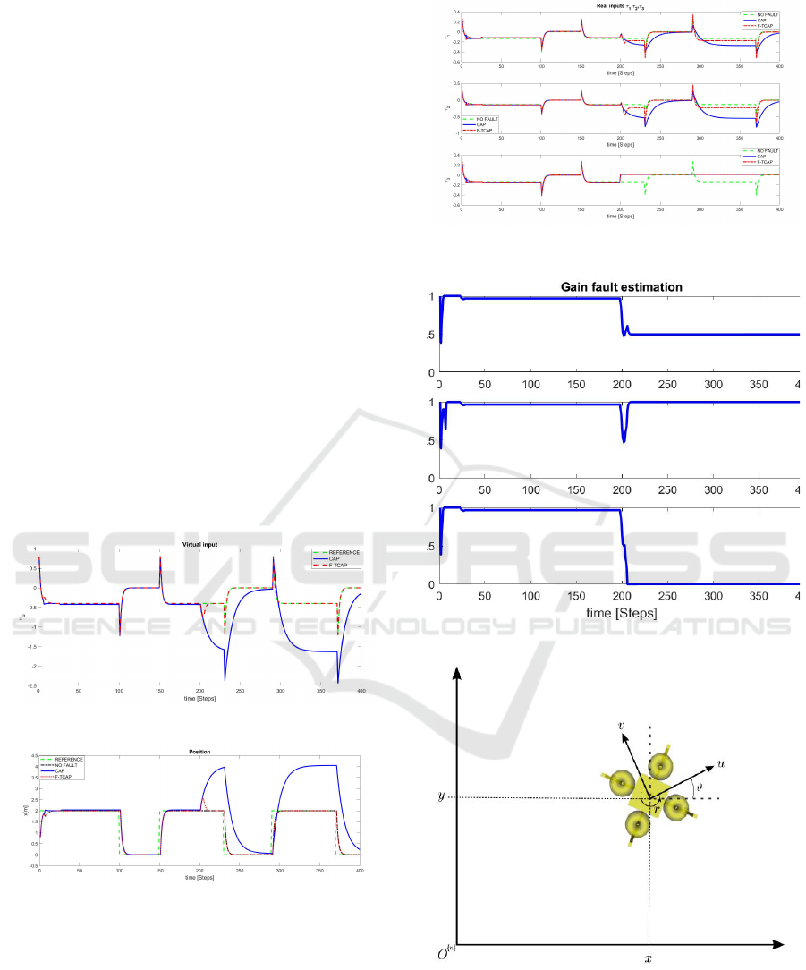
In Figure 2, the virtual signals are shown in three

different cases i.e No fault, CAP, and F-TCAP. This

shows that the control law is not disturbed by the

faulty actuator. In Figure 3, the position vector is

plotted. Here, it can be noticed that the F-TCAP algo-

rithm successfully tracks the reference position under

actuator and bias faulty events. It is observed that a

small perturbation is generated in the case of F-TCAP,

while the behavior of the CAP method is highly dis-

turbed by faulty events. Figure 4 reports the physical

inputs. This shows that the signals of faulty actua-

tor smartly changed- all signals are distributed among

healthy actuators after the actuator got stuck. In last,

Figure 5 shows the loss of effectiveness parameters.

Notice in this viewpoint, the F-TCAP algorithm tol-

erates the fault better than the CAP algorithm.

Figure 2: Virtual inputs.

Figure 3: Position.

4.2 Marine Surface Vehicle

In this section, we consider the surface marine vehicle

depicted in Figure 6. The model and the control struc-

ture are taken from (Folino, 2018; D’Angelo, 2018).

There, the system position is denoted by η = [x,y,θ]

where x and y are earth-ﬁxed positions and θ is the

yaw angle. The body-ﬁxed velocities are denoted

with ρ = [u,v,r]

where u is forward velocity, v is lat-

Figure 4: Physical inputs: τ

= u

+ f

Figure 5: Fault loss of effectiveness proﬁles.

Figure 6: Schematic model of the ship.

eral velocity, and r is yaw angular velocity. The thrust

and force moment of the vehicle are represented by

υ = [υ

,υ

]

and are generated via the thrust vec-

tor τ = [τ

,τ

]

as depicted in Figure 7. More

formally the kinematic model of the system is given

ICINCO 2020 - 17th International Conference on Informatics in Control, Automation and Robotics

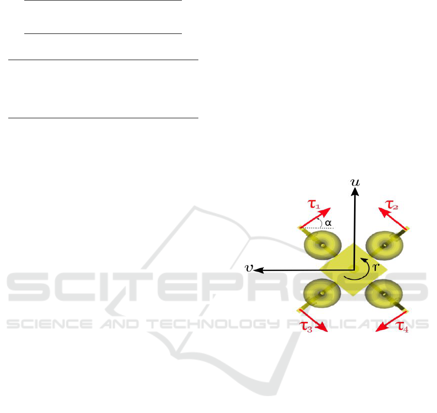
Table 1: The system matrices.

M Inertia matrix

C Coriolis/centripetal matrix

D Hydrodynamics damping matrix

Table 2: Parameters deﬁnitions.

m = 1.1274 [Kg] Mass

= 1[Kg m

] moment of Inertia

= 0.0414[Kg/m] friction force coefﬁcient along u

= 0.0414[Kg/m] friction force coefﬁcient along v

= 0.0568[Kg m

] friction torque coefﬁcient along r

α = π/4 thruster angle in the body frame

as follows:

η(t) = R(θ(t))ρ(t) (18)

where R(θ) is the rotational matrix around the yaw

angle deﬁned as

R(θ) :=





cos(θ) −sin(θ) 0

sin(θ) cos(θ) 0

0 0 1





while the dynamic model is derived as:

ρ(t) +C(ρ(t))ρ(t) + D(ρ(t))ρ(t) = υ(t) (19)

where the system matrices, whose meaning and nu-

merical parameters are reported in Tables 1-2, take

the following form:

M :=





m 0 0

0 m 0

0 0 I





C(ρ) :=





0 −mr 0

mr 0 0

0 0 0





D(ρ) :=





u 0 0

0 β

v 0

0 0 β





Such a model can be recast as:

ρ(t) = A(ρ(t)) +

υ(t) (20)

that is more similar to (3) although in continuous-time

domain. Here the matrix A(ρ(t)) := −M

−1

(C(ρ(t))+

D(ρ(t))ρ(t), while

:= M

−1

. Thus,the discrete-time

state-space representation (3) takes the form:



η(t + 1)

ρ(t + 1)





I T

R(θ(t))

0 I + T

−1

(C(ρ(t)) + D(ρ(t))





η(t)

ρ(t)







υ(t)

where T

is the sampling period and B

= T

In particular input υ is produced by the 4 thrusters

according to the following allocation law

υ(t) = B

τ(t) (21)

where the allocation matrix B

is deﬁned as:





sin(α) sin(α) − sin(α) −sin(α)

cos(α) −cos(α) cos(α) −cos(α)

−l/2 l/2 l/2 −l/2





(22)

In (21) τ

and τ

denote the signals for two identical

main propellers and τ

and τ

are the control signals

for the transverse thrusters. In this respect τ repre-

sents the signal generated by the actuators on the basis

of the physical input u(t) = [u

]

produced

by the allocation unit according to the following ex-

pressions that accounts also for possible faulty events

τ(t) = ∆(t)u(t) + f (t) (23)

where ∆ ∈ R

4×4

represents the control effectiveness

matrix and f (t) models bias faults.

Figure 7: Thrust forces allocation.

In view of the previous discussion, the signal υ can

be considered as the virtual control signal. It is deter-

mined by the following time-invariant control law

υ(t) = K

(θ(t))K

(η

(t) − η(t)) − ρ(t)] (24)

where the controller gains are K

= 0.75I

3×3

, K

0.63I

3×3

and η

(t) is the desired trajectory to track.

The sampling period for both the control law and the

control allocator is T

= 0.2827.

The goal of the ﬁrst simulation campaign is to suc-

cessfully allocate virtual law (24) with desired refer-

ence η

evolving as











[0,0,0]

for t < 12

[2,0,0]

for 12

≤ t ≤ 200

[2,2,π]

for 200

< t ≤ 500

[0,0,0]

for t > 500

(25)

under the constraints

−0.1 ≤ u

≤ 0.1and − 0.09 ≤ u

− u

(t − 1) ≤ 0.09

(26)

Adaptive Fault-Tolerant Control Allocation Schemes for Overactuated Systems with Actuator and Bias Faults

and despite the matrix effectiveness and bias actuator

faults assumed as:

∆(t) = diag{1,1, 1, 1}for t < 12

∆(t) = diag{0.9,1,1,1}for 12

≤ t ≤ 200

∆(t) = diag{0.8,1,0,1}for t > 200

(27)

f (t) = [0,0,0,0]

for t < 12

f (t) = [0.01,0,0,0]

for 12

≤ t ≤ 200

f (t) = [0,0,0.01,0]

for t > 200

(28)

In particular note that after t > 200

, the third actuator

gets stuck until the simulation.

In order to show the effectiveness of the proposed

scheme, we have simulated the model under the fol-

lowing scenarios:

• No Fault: the model is simulated without consid-

ering any fault.

• CAP: the algorithm is implemented without cal-

culation of effectiveness matrix and bias fault es-

timation.

• F-TCAP: the algorithm is simulated with the cal-

culation of effectiveness matrix and bias faults es-

timation.

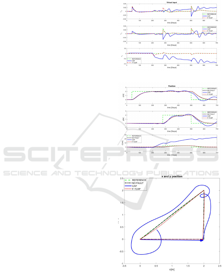
The results of this ﬁrst simulation are reported in Fig-

ures 8-12. In particular Figure 8 shows the total vir-

tual control input needed to drive the vehicle. It is

observed that the virtual control inputs are success-

fully tracked and the system remains bounded with

smooth variations by using the F-TCAP algorithm.

Figures 9 and 10 show the positions of the vehicle

by using CAP and F-TCAP algorithm. The simula-

tion results demonstrate that the variables continue to

track their desired values after a fault occurs by using

the F-TCAP algorithm while the CAP is not working

correctly. It is observed that the system remains stable

under faulty conditions with F-TCAP. The physical

inputs are plotted in Figure 11. The proposed algo-

rithm successfully allocates the control efforts to the

vehicle under faulty scenarios and distributes the con-

trol to the healthy actuators. Figure 12 gain fault es-

timation. Here, the loss of effectiveness parameters is

estimated and plotted. The system shows a small per-

turbation when the fault occurs. It is observed that the

proposed algorithm performed better in case of recon-

ﬁguration and control allocation as compared to the

CAP algorithm under actuator faults, rate constraints

and bias faults.

A second simulation example has been performed

to observe the behaviour of the CAP and F-TCAP al-

gorithms when the vehicle ﬁxed is instructed to keep

position at a ﬁxed point when an actuator is stuck. In

Figure 8: Example 1: Virtual inputs.

Figure 9: Example 1: Vehicle positions and angle.

Figure 10: Example 1: x and y position of the vehicle.

this example, we assumed a reference path position

as η

(t) = [0,0,0]

,∀t ≥ 0. During the simulation,

the actuator fault ∆(t) = [1,0,1,1]

and bias fault as

f (t) = [0,0.8,0,0]

is imposed on the model in the

ICINCO 2020 - 17th International Conference on Informatics in Control, Automation and Robotics

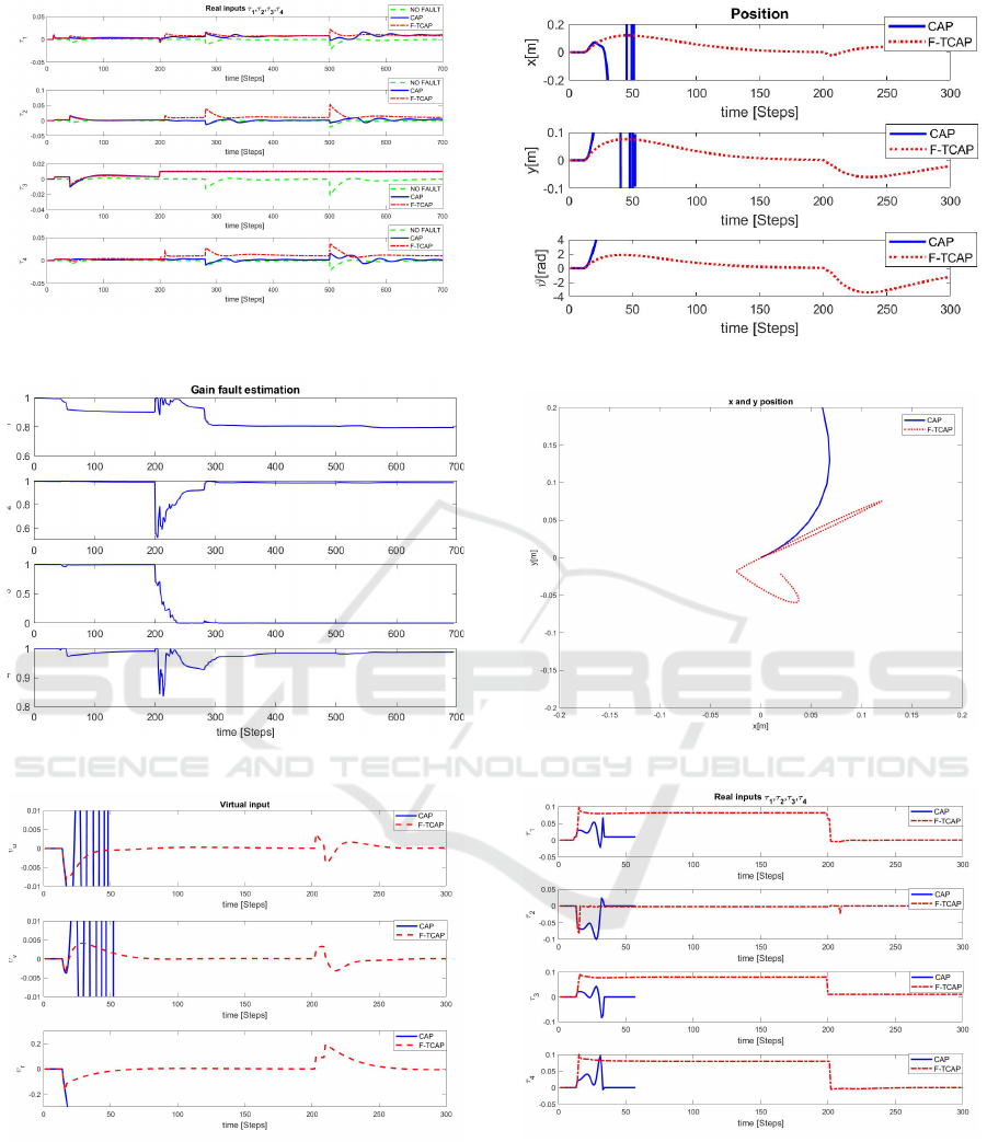
Figure 11: Example 1: Physical inputs.

Figure 12: Example 1: Fault loss of effectiveness proﬁles.

Figure 13: Example 2: Virtual inputs.

time range 12

≤ t ≤ 200

. Figure 13 shows the vir-

tual control input that is used to generate the physical

inputs as shown in Figure 16. The position of the ve-

hicle is shown in Figure 14 and 15. It can be noted

that under CAP the vehicle position goes to inﬁnity.

On the contrary, under F-TCAP the vehicle remains

close to the reference position thanks to the action of

Figure 14: Example 2: Vehicle positions and angle.

Figure 15: Example 2: x and y position of the vehicle.

Figure 16: Example 2: Physical inputs.

the allocation unit. This depicts that the vehicle is

stable and input signals are bounded by using the F-

TCAP algorithm under actuator and bias faults.

Adaptive Fault-Tolerant Control Allocation Schemes for Overactuated Systems with Actuator and Bias Faults

5 CONCLUSIONS

In this paper, a new adaptive fault-tolerant control

allocation algorithm is proposed. The proposed al-

gorithm integrates online effectiveness matrix and

bias faults estimation with the control allocation al-

gorithm. The actuator and bias faults are considered

under actuator amplitude and rate constraints. The ef-

fectiveness of the proposal is shown by using a marine

surface vehicle model where the proposed algorithm

showed good performance in terms of control allo-

cation. Future works foresees the implementation of

this class of adaptive control allocation strategies on

real redundant marine vehicles.

ACKNOWLEDGEMENTS

The authors want to thank Ing. Paolo Folino and Ing.

Vincenzo D’Angelo by AppliCon S.r.l for providing

us with the mathematical model of the autonomous

marine vehicle they developed in their master’s the-

ses and for useful discussions and assistance in their

vehicle control and guidance aspects.

REFERENCES

Casavola, A. and Garone, E. (2010). Fault-tolerant adaptive

control allocation schemes for overactuated systems.

International Journal of Robust and Nonlinear Con-

trol, 20(17):1958–1980.

Chu, Z., Xiang, X., Zhu, D., Luo, C., and Xie, D. (2018).

Adaptive fuzzy sliding mode diving control for au-

tonomous underwater vehicle with input constraint.

International Journal of Fuzzy Systems, 20(5):1460–

1469.

D’Angelo, V. (2018). Strategie di gestione delle missioni

e controllo di un veicolo marino autonomo di superﬁ-

cie. Master’s thesis, University of Calabria. Master’s

thesis in Automation Engineering.

Folino, P. (2018). Strategie di guida e navigazione per un

veicolo marino autonomo di superﬁcie. Master’s the-

sis, University of Calabria. Master’s thesis in Automa-

tion Engineering.

He, C., Feng, Z., and Ren, Z. (2012). Flocking of multi-

agents based on consensus protocol and pinning con-

trol. In Proceedings of the 10th World Congress on In-

telligent Control and Automation, pages 1311–1316.

IEEE.

Ismail, Z. H., Faudzi, A., and Dunnigan, M. W. (2014).

Fault-tolerant region-based control of an underwater

vehicle with kinematically redundant thrusters. Math-

ematical Problems in Engineering, 2014.

Khan, H. Z. I., Rajput, J., Ahmed, S., Sarmad, M., and

Sharjil, M. (2018). Robust control of overactuated au-

tonomous underwater vehicle. In 2018 15th Interna-

tional Bhurban Conference on Applied Sciences and

Technology (IBCAST), pages 269–275. IEEE.

Liu, X., Zhang, M., and Yao, F. (2018). Adaptive fault

tolerant control and thruster fault reconstruction for

autonomous underwater vehicle. Ocean Engineering,

155:10–23.

Patel, H. R. and Shah, V. A. (2018). A framework for fault-

tolerant control for an interacting and non-interacting

level control system using ai. In ICINCO (1), pages

190–200.

Tohidi, S. S., Yildiz, Y., and Kolmanovsky, I. (2016). Fault

tolerant control for over-actuated systems: An adap-

tive correction approach. In 2016 American Control

Conference (ACC), pages 2530–2535. IEEE.

Tohidi, S. S., Yildiz, Y., and Kolmanovsky, I. (2017). Adap-

tive control allocation for over-actuated systems with

actuator saturation. IFAc-PapersOnLine, 50(1):5492–

5497.

Wang, B. and Zhang, Y. (2017). An adaptive fault-

tolerant sliding mode control allocation scheme for

multirotor helicopter subject to simultaneous actuator

faults. IEEE Transactions on Industrial Electronics,

65(5):4227–4236.

Wang, Y., Wilson, P. A., Liu, X., et al. (2015). Adaptive

neural network-based backstepping fault tolerant con-

trol for underwater vehicles with thruster fault. Ocean

Engineering, 110:15–24.

Zhang, M., Liu, X., and Wang, F. (2017). Backstepping

based adaptive region tracking fault tolerant control

for autonomous underwater vehicles. The Journal of

Navigation, 70(1):184–204.

ICINCO 2020 - 17th International Conference on Informatics in Control, Automation and Robotics