A CART-based Genetic Algorithm for Constructing Higher Accuracy

Decision Trees

Elif Ersoy

, Erinç Albey

and Enis Kayış

Department of Industrial Engineering, Özyeğin University, 34794, Istanbul, Turkey

Keywords: Decision Tree, Heuristic, Genetic Algorithm, Metaheuristic.

Abstract: Decision trees are among the most popular classification methods due to ease of implementation and simple

interpretation. In traditional methods like CART (classification and regression tree), ID4, C4.5; trees are

constructed by myopic, greedy top-down induction strategy. In this strategy, the possible impact of future

splits in the tree is not considered while determining each split in the tree. Therefore, the generated tree cannot

be the optimal solution for the classification problem. In this paper, to improve the accuracy of the decision

trees, we propose a genetic algorithm with a genuine chromosome structure. We also address the selection of

the initial population by considering a blend of randomly generated solutions and solutions from traditional,

greedy tree generation algorithms which is constructed for reduced problem instances. The performance of

the proposed genetic algorithm is tested using different datasets, varying bounds on the depth of the resulting

trees and using different initial population blends within the mentioned varieties. Results reveal that the

performance of the proposed genetic algorithm is superior to that of CART in almost all datasets used in the

analysis.

1 INTRODUCTION

Classification is a technique that identifies the

categories/labels of unknown observations/data

points, and models are constructed with the help of a

training dataset whose categories/labels are known.

There are many different types of classification

techniques such as Logistic Regression, Naive Bayes

Classifier, Nearest Neighbor, Support Vector

Machines, Decision Trees, Random Forest,

Stochastic Gradient Descent, Neural Networks, etc.

Classification techniques are divided into two groups:

(1) binary classifiers that classify two distinct classes

or two possible outcomes and (2) multi-class

classifiers that classify more than two distinct classes.

Also, many of these methods are constructed with a

greedy approach. Hence, these approaches always

make the choice that seems to be the best at each step.

However, these greedy approaches may not result in

an optimal solution.

Decision trees (DT) are one of the most widely-

used techniques in classification problems. They are

https://orcid.org/0000-0003-1126-213X

https://orcid.org/0000-0001-5004-0578

https://orcid.org/0000-0001-8282-5572

guided by the training data (x

, y

), i = 1, . . . , n.

(Bertsimas and Dunn, 2017). DTs recursively

partition the training data’s feature space through

splits and assign a label(class) to each partition. Then

created tree is used to classify future points according

to these splits and labels. Since, conventional decision

tree methods are creating each split in each node with

greedy approaches and top-down induction methods,

which may not capture well the underlying

characteristics of the entire dataset. The possible

impact of future splits is not considered while

determining each split in the tree. Thus, attempts to

construct near-optimal decision trees have been

discussed for a long time (Safavian and Landgrebe,

1991).

The use of heuristics in creating decision trees

with the greedy approach is discussed widely in the

literature. Heuristic algorithms will be applied to

construct decision trees from scratch or to improve

the performance of constructed trees. Kolçe and

Frasheri (2014) study on the greedy decision trees and

focus on four of the most popular heuristic search

328

Ersoy, E., Albey, E. and Kayı¸s, E.

A CART-based Genetic Algorithm for Constructing Higher Accuracy Decision Trees.

DOI: 10.5220/0009893903280338

In Proceedings of the 9th International Conference on Data Science, Technology and Applications (DATA 2020), pages 328-338

ISBN: 978-989-758-440-4

algorithms, such as hill-climbing, simulated

annealing, tabu search, and genetic algorithms (Kolçe

and Frasheri, 2014). For continuous feature data,

evolutionary design is suggested in Zhao and

Shirasaka (1999) and an extreme point tabu search

algorithm is proposed in Bennett and Blue (1996).

There are some examples for optimal decision

trees. For example, Blue and Bennett (1997) use a

Tabu Search Algorithm for global tree optimization.

In their paper, they mention that “Typically, greedy

methods are constructed one decision at a time

starting at the root. However, locally good but

globally poor choices of the decisions at each node

can result in excessively large trees that do not reflect

the underlying structure of the data”. Gehrke et al.

(1999), develop a bootstrapped optimistic algorithm

for decision tree construction.

The genetic algorithm (GA) have been proposed

to create decision trees in the literature and have been

discussed in two different ways to find near-optimal

decision trees. One method is for selecting features to

be used to construct new decision trees in a hybrid or

preprocessing manner (Bala et al., 1995) and others,

applies algorithm directly to constructed decision

trees to improve them (Papagelis and Kalles, 2000).

Also, additionally, Chai et al. (1996) construct a

linear decision binary tree with constructing

piecewise linear classifiers with the GA. Therefore,

we choose to use a GA to construct highly accurate

decision trees to expand the search area so as not to

get stuck in local optima and get close to the near-

optimal tree.

In GA literature, different approaches are used to

construct an initial population. Most of them use

randomly generated populations (Papagelis and

Kalles, 2000; Jankowski and Jackowski, 2015) and

some of them use a more intelligent population with

the help of greedy algorithms (Fu et al., 2003; Ryan

and Rayward-Smith, 1998). In Fu et al. and Ryan et

al.’s works, C4.5 is used as a greedy algorithm to

construct the initial population. An intelligent

population helps to start the algorithm with better

fitness values. Also, in their paper, they discussed that

using C4.5 is a bit computationally expensive.

In this work, we develop a GA to construct high

accuracy decision trees. Also, we use greedy

algorithm CART trees in the initial population to

improve these trees’ performance. In GA, to

implement evolutionary operations, decision trees

must be represented as chromosome structures. In this

work, we propose a structure to encode a decision tree

to a chromosome and to generate the initial

population, we divide the original dataset into subsets

with reasonable size and generate trees with these

subsets on CART. Then in GA full-size dataset and

the initial population are used to create more accurate

trees. So, we want to use the power of CART trees in

our algorithm and we are trying to improve the

performance of greedy CART solutions.

The rest of the paper is organized as follows. In

Methodology section, you can find a more detailed

explanation of our implementation of GA,

chromosome structure and generated initial

populations. Subsections of the Methodology section

present the encoding/decoding decision trees to/from

chromosomes, genetic operators like mutation and

crossover, fitness functions. Experiment and

Computational Result section explains the

experimental details and results. Finally, Conclusion

section concludes all of this work.

2 GENETIC ALGORITHM AS A

SOLUTION METHOD

In this paper, we discuss GA to improve the

performance of decision trees. For the GA

implementation, we concentrate on the following

facts: (1) new chromosome structure, (2) initial

population, (3) fitness function, (4) selection

algorithm, (5-6) genetic operations, (7) generation

and (8) stopping condition and overall flow of GA.

These are explained in detail in following subsections

to understand the essentials of our GA.

2.1 Encoding the Solution

Representation (Chromosome

Structure)

The representation of a solution using the

chromosome is critical for relevant search in solution

space and tree-based representation for the candidate

solution is the best one (Jankowski and Jackowski,

2015). A chromosome must contain all split decisions

and rules to decode it into a feasible decision tree.

Figure 1: Tree structure and split rules at depth 3.

A CART-based Genetic Algorithm for Constructing Higher Accuracy Decision Trees

329

Decision trees are constructed based on split rules

and in each node, split occurs with a rule, and data-

points are following the related branch based on that

rule. Also, in this paper, we concentrate on binary

split trees so there are only two branches in each node

splits, which means splits are bidirectional. Left

branch refers less than operation and the right branch

refers greater than or equal to operation (see Figure

1). So, in GA’s solution representation if we encode

which feature is used as a rule in which branch node,

and their threshold values we will construct a tree

with this linear representation. Then the fitness value

will be calculated easily. To encode that

representation, we use a modification of Jankowski

and Jackowski (2015) as follows.

𝑎



𝑎



𝑎



𝑎



𝑎



𝑎



𝑎



𝑏



𝑏



𝑏



𝑏



𝑏



𝑏



𝑏



Figure 2: Chromosome structure for depth 3 tree.

Each branch node is stored in a depth-first manner

as an implicit data structure in two arrays (see Figure

2). All feature IDs are maps to an integer and each

feature values are maps to normalized continuous

values between [0,1], so each component is numeric.

The dimension of a chromosome is 2x(2

-1). We

use 2 rows where first-row stores split feature

information and second-row stores threshold values

for the related feature. Number of columns equal to

the number of total branch nodes, 2

-1, where D is

the depth of a tree. Also, in our algorithm D is used

as a fixed parameter, thus chromosome dimension is

also fixed. We define a tree if and only if the right

branch always follows the “>=” rule and left branch

follow “<” rule. Thus, if the related feature of the

node’s rule and the threshold for that rule is known,

they are enough to construct a tree easily. So, the

chromosome structure of depth 3 is presented below.

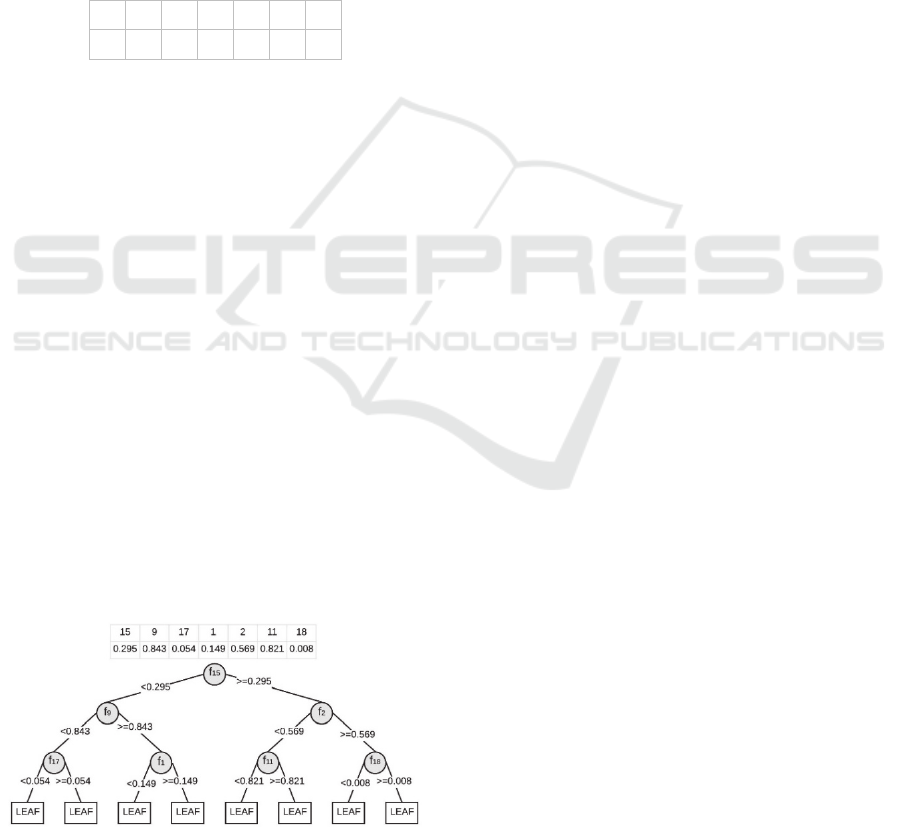
One of the decision trees at depth 3 is represented

in Figure 3. To explain it in detail, split feature at the

root node is 15

feature and threshold is 0.295. So, in

Figure 3: Example chromosome and related decision tree at

depth 3.

training data, datapoints whose 15

feature is less

than 0.295, follow left branch, accumulated in node 2

and points greater than or equal to 0.295, follow right

branch and accumulated in node 5. Second column of

the chromosome represents the rule of left node, node

2, then split feature is 9

feature and threshold is

0.843. Thus, data points accumulated in node 2

follows that rule, they are split according to their 9

feature and if the value is less than 0.843 they follow

left branch, accumulated in node 3 and points greater

than or equal to 0.843 follows right branch and

accumulated in node 4. Then 3

column of the

chromosome is the left branch of the node 2 and split

feature is 17

one, threshold is 0.149. Then if 17

features of data points in the node 2 are less than

0.149 datapoints assign to Leaf #1 and others assign

to Leaf #2.

2.2 Generation of Initial Population

To generate initial solutions/populations for the GA,

CART (Breiman et al., 1984) is used as a constructive

algorithm. But GA needs an initial population that has

more than 1 solution, so as Fu et. al (2003) used in

their paper, some sub-trees are created for the initial

population. In this paper, we generate sub-trees using

two ways: randomly and with the CART algorithm.

For random trees, we generate a tree with randomly

chosen features for each node of a tree with given

depth and random threshold values within the

normalized values between 0 and 1. For sub-CART

trees, a whole size data set is divided into some

number of subsets randomly with a decided instance

size (explained in Section 3.3) and CARTs are

generated for these subsets. Some data points can be

in multiple subsets. When subsets of this dataset are

used in CART, a solution will be found for these

subsets and we call them as sub-trees. Then original

data will be classified using these subtrees and fitness

value for each subtree is calculated for the whole

dataset. Fitness is defined as the total

misclassification error, which will be discussed in

more detail later.

We use two different initial population mixtures

(1) random trees only and (2) random trees, subtrees

generated via CART, and 1 full CART solutions.

Details for these population types and effects of these

selections are discussed in Section 3.

2.3 Fitness Value

Fitness Value will be calculated as total number of

misclassified points or total correctly classified points

of each individual tree. A misclassification is number

DATA 2020 - 9th International Conference on Data Science, Technology and Applications

330

of points that are labeled incorrectly. In other words,

in classification trees, leaf nodes are labeled with the

majority points’ class labels after split rules.

Therefore, other minority points are labeled

incorrectly, and the total number of that minority

points is equal to the misclassification error and

others are labeled correctly. Aim of our algorithm and

all other classification algorithms are minimizing

number of misclassification or maximizing number of

correctly classified points, which are almost the same

things.

In our algorithm, we choose maximizing correctly

classified points as an objective. Thus, our fitness

value is equal to total number of correctly classified

points. We choose this one because of the working

principle of our selection algorithm, we explain it in

the following section in more detail.

When a new tree is reproduced after evolutionary

operations, fitness value needs to be updated. Firstly,

points are assigned to related leaf nodes according to

new split rules. Then, each leaf is labeled with

majority class, we call poin ts labeled incorrectly

according to their real class labels, as misclassified

points and others labeled as correctly classified

points.

In the GA algorithm, we calculate the fitness

function value of each individual sub-tree with the

whole dataset instead of the related subset, because,

in this paper, the classification tree must be generated

for the whole dataset which considers all data points

completely.

2.4 Parent Selection

In GA, during children production, the algorithm uses

the current generation to create children that make up

the next generation based on the fitness value. In GA

and other evolutionary algorithms, to select parents,

some well-known selection methods are tournament

selection, roulette wheel selection, rank-based

selection, etc. In these selection methods, each

individual in the population can be selected more than

once, so each individual spread its genes to possibly

more than one child.

In our implementation of the GA, we use roulette

wheel (RW) selection. Roulette wheel selection is

under the title of Fitness Proportionate Selection

Methods. In these methods, every solution has a

probability of being selected according to their fitness

values proportion. In roulette wheel, fitness values of

each tree in the current generation take a place in the

wheel according to their weighted fitness value. Thus,

higher fitness takes wider proportion and it will be

selected with a higher probability. Furthermore, we

want to choose high accuracy trees as a parent to

spread its genes to the next generations. This will help

us to reproduce stronger children. If fitness value is

used as a total number of correctly classified points,

the roulette wheel works well and will chooses high

accurate trees with higher probability. So, to select

stronger parents, which has less number of misclassed

points and more correctly classified ones, roulette

wheel method is the proper one. That’s why we

choose our objective as maximize fitness function

which is total number of correctly labeled points.

2.5 Crossover Operation

The algorithm creates crossover children by

combining pairs of selected parents in the current

population. Firstly, two individuals (parents) are

chosen using the RW method. From chosen trees, a

random cut point is selected according to a randomly

generated number which can take values between 1

(root node) to n (total number of tree nodes). After

identifying the random cut points in both parents, new

individuals (offspring) are created by replacing sub-

part form the first parent by the one from the second

parent. We cut each parent from the exact same

point/node and replace the remaining part with a same

sized sub-parts. Figure 6 illustrates an example of the

crossover operation.

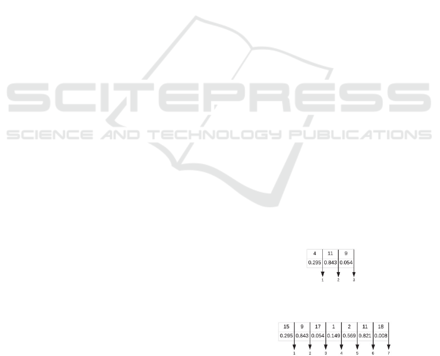
Also, in this paper’s algorithm, crossover is applied on

linear chromosome in two ways, 1-point, and 2-point

crossover. In 1-point crossover, the sub-part starting from

the cutting node (and runs through the last node of the

selected parent) is exchanged; whereas in 2-points

crossover, we exchange interior sub-parts. In more detail,

we cut sub-trees at the same level from each parent. In

Figure 4, possible cut points for depth 2 trees are shown. 1-

point crossover is applied when parents are cut from the 1

or 2

cut points and crossed each other. 2-point crossover

is applied when the part between the 1

and 2

cut point

Figure 4: Possible crossover cut points in depth 2; 1 or 1-2

or 2.

Figure 5: Possible crossover cut points in depth 3; 1 or 1-4

or 2-3 or 3-4 or 4 or 5-6 or 6.

A CART-based Genetic Algorithm for Constructing Higher Accuracy Decision Trees

331

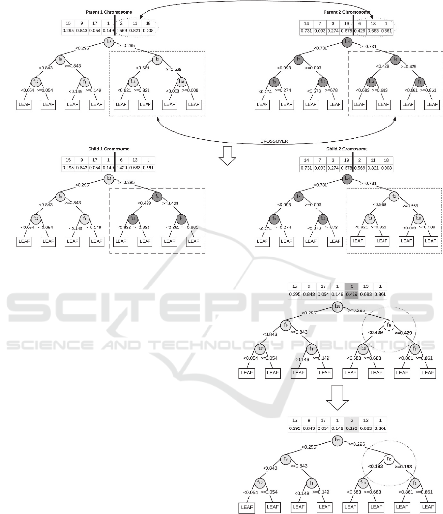
Figure 6: Crossover operation on selected parent and generated children in depth 3 trees.

is crossed. To be more precise, after the crossover

operation, depth of the tree cannot change because we

cut each parent from the exact same point. Figure 5

shows cut points for depth 3. For 1-point crossover at

depth 3, possible cut points will be 1, 4 or 6 and for

2-point crossover, possible parts will be between 1-4,

2-3, 3-4 or 5-6. These specific cut-parts represent

each meaningful sub-tree in a maximal tree. This

specification also prevents depth change in the

crossover.

In Figure 6, you can see the illustration of 1-point

crossover on the depth 3 tree. We cut each parent

from the 4

cut point, which is decided randomly in

the algorithm, and cut parts crossing between each

other.

2.6 Mutation Operation

Mutation operation makes changes on the individual

tree in the population. In the proposed algorithm, this

change is applied, based on mutation rate, on to the

generated children`s randomly selected node to create

a mutated child. With the help of mutation, GA

enables us to search a broader space with providing

genetic diversity. In our implementation, we use node

base mutation similar to Jankowski and Jackowski

(2015), we randomly change both feature and split

threshold of a randomly selected node (see Figure 7).

Figure 7: Tree node mutation.

Figure 7 illustrates how mutation operation

applied on Child 1, which comes from the crossover.

In this mutation, 5

node is selected randomly, and

this node’s feature ID and threshold value are

changed with randomly chosen feature ID and

threshold value. With mutation, the class assignment

DATA 2020 - 9th International Conference on Data Science, Technology and Applications

332

of leaf nodes may also change based on the majority

class on each node because split rule is changed. Also,

there is a restriction, mutation will be applied to all

branch nodes except the root node.

2.7 Replacement and New Generation

To generate a new generation of the GA, we applied

the elitism procedure. Elitism keeps a proportion

known as elite rate, of the fittest candidates into the

next generation. For example, given a population of

100 individuals, if you have an elite rate of 5%, you

choose to keep the five best individuals of the current

generation to the next generations and you apply

crossover and mutation to generate the rest of the new

generation.

2.8 Stopping Criteria and Overall

Algorithm

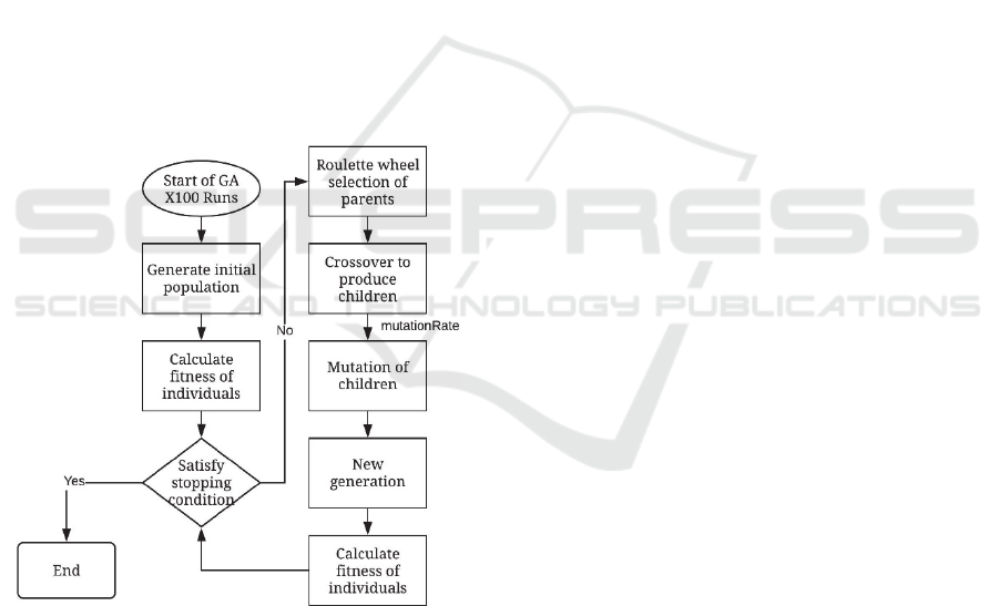
In the literature, there are many different applications

of GA implementation. The flowchart in Figure 8

shows the general steps of our GA implementation.

Figure 8: Flow of GA.

To explain our algorithm in more detail, the steps

of GA implementation is as follows:

Repeat below steps TotalRun times:

 Generate an initial population (first generation)

of size N with the selected mixture.

 Initialize a variable, Iter, for keeping track of

successive iterations where the best tree found in

each generation has not changed.

 Repeat while Iter < MaxIter:

o Select eliteRate*N best individual from

the previous generation and keep them

into the new generation.

o Repeat until the new generation is

fulfilled to size N.

- Randomly select two members from

the previous generation based on

roulette wheel method.

- Run the crossover operator: input

selected two members and obtain two

children.

- Add new children to the new

generation

- Run the mutation operator: input one

of the currently generated children

from crossover and apply mutation if

mutationRate is satisfied.

- Replace mutated child in the new

population.

- If the new generation cannot provide

a better tree and fitness value than the

previous generation’s best, increase

Iter by 1.

 Select the best tree in the final generation

and its fitness.

We repeat these steps TotalRun times in order to

minimize the effects of randomization on overall

performance. Also, we choose the final solution as the

best tree found in all TotalRun runs.

3 COMPUTATIONAL RESULTS

In this section, we explain our datasets, parameters,

initial populations, then the computational results of

the proposed approach on different variations of

datasets are discussed. We compare the performance

of our GA to that of CART.

3.1 Datasets

To evaluate the effects of data size, number of

features and class we use six different datasets with

different dimensions and characteristics. These

datasets are obtained from the UCI machine learning

repository (Lichman, 2013). Some of these datasets

are used in other classification studies as well, such

as study about optimal classification tree (Bertsimas

and Dunn, 2017). Details about each dataset are

described below (see Table 1).

A CART-based Genetic Algorithm for Constructing Higher Accuracy Decision Trees

333

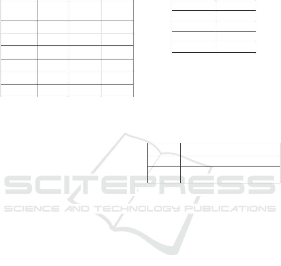
Table 1: Details of datasets used in experiments.

Data Set

Name

Number of

Points (n)

Number of

Classes (K)

Number of

Features (p)

Wine 173 3 13

Chess 3196 2 36

Image

Segmentation

210 7 19

Avila 20867 12 10

Parkinson 756 2 754

Madelon 2600 2 500

We are given each dataset to GA in the form of

(X, Y). To be more general, each dataset containing n

observations, each observation is defined with p

features and K possible class label. The x values for

each feature across the data are normalized between

0 and 1, which means each x

∈

[0, 1]

We apply 5-fold cross-validation to estimate the

performance of our algorithm to minimize the

overfitting problem. We split each dataset as 80% for

training and 20% for testing sets. And then we take

an average of 5 runs` accuracies.

3.2 Parameters

In our proposed GA, we use four parameters: (1)

maxIter which is used for restricting the ineffective

improvement moves to stop algorithm, (2) Elite Rate

represents the proportion of best individual to keep in

next generation, (3) Mutation Rate is the proportion

for mutation operation applied on children and (4)

TotalRun which is the total number of replications.

For maxIter, in each ineffective generation, iteration

counter increases but if the new generation improves

the best solution and updates the best tree so far,

iteration does not increase and iteration counter is

reset. If the iteration counter reaches maxIter, GA

terminates. We take TotalRun amounts of replications

because, in the applied algorithm, there are lots of

randomization in reproduction operators as selection,

crossover and mutation. So, we apply some

replications and decrease the effect of randomness

over each procedure. In this work, we use the

parameter values as shown in Table 2. Sensitivity

analysis is applied to these parameters and final

values are selected as the values that yield the best

performance.

Table 2: Values of each parameter.

Parameter Value

MaxIter 10

Elit Rate 0.2

Mutation Rate 0.1

Total Run 100

3.3 Initial Population

As mentioned before, this work aims to improve the

performance of GA by using a specific initial

population. We use two different population blends

for initializing our algorithm. These mixtures include

random trees, sub-CART trees which are generated

with sub-sets of the whole datasets and 1 CART tree

which is constructed with the full-size training set.

Table 3: Content of population blends.

Population Content

MIX_V1 30 Random Trees

MIX_V2

30 Random + 30 Sub-CART + 1 full-

CART Trees

We generate each random tree by assigning

random rules for a given depth. Random feature ID

for each node, which is integer, is assigned between

[0, p] and threshold value, which is continuous,

between [0,1]. For constructing CART trees, we used

the rpart package (Therneau et al. 2019) in the R

programming language version 3.5.3 (R Core Team

2019). In the rpart function, there is a control

parameter called minbucket, which limits the

minimum number of observations in any leaf node to

prevent overfitting. We use this parameter as

(0.05*n).

We add CART based decision trees into the initial

population and our aim is to beat CART

performances with the help of GA. We will evaluate

the contributions of CART based initial population in

the next subsection.

3.4 Experimental Analysis and Result

As mentioned in previous subsections, we use 6

different datasets with different sizes, and we divide

them into 5 folds. We aim to find more accurate trees

rather than the CART. As an initial population, we

use 2 different population mixtures with different size

(see Table 3).

DATA 2020 - 9th International Conference on Data Science, Technology and Applications

334

Our first initial population includes 30 different

random trees with a given depth. And second initial

population type includes the same 30 random trees

plus 30 sub-CART and 1 full-sized CART solution.

Also, we train each dataset at 4 different depths as {2,

3, 4, 5}.

We take 100 replication runs to minimize effects

of randomization. So, to compare our GA results we

take best tree found in overall 100 runs as a final

solution. In the below tables, “mean out-sample

accuracy” is refer to average out-sample accuracy of

the best tree found in 100 runs of 5 folds.

We use average out-sample accuracies across 5

folds to compare the performance of our algorithm

against CART in cross-validation manner. Also, to

show the exact improvement performance of our

Table 4: Full results at depth 2.

DATASET

Mean Out-Sample

Accuracy

Mean In-Sample

Accuracy Improvement

Time(sec)

Wine

CART 88.78% 0.112

GA MIX_V1 88.19% +12.22% 0.460

GA MIX_V2 88.21% +2.67% 0.767

Chess

CART 76.69% 0.131

GA MIX_V1 86.64% +17.47% 7.543

GA MIX_V2 86.92% +0.52% 7.700

Segment

CART 37.14% 0.169

GA MIX_V1 57.14% +8.10% 0.566

GA MIX_V2 58.10% +3.10% 0.645

Avila

CART 50.10% 0.257

GA MIX_V1 51.14% +3.14% 32.721

GA MIX_V2 51.97% +0.78% 41.768

Parkinson

CART 79.89% 0.349

GA MIX_V1 79.10% +2.71% 1.697

GA MIX_V2 81.88% +0.07% 1.872

Madelon

CART 65.19% 0.783

GA MIX_V1 57.00% +5.45% 7.248

GA MIX_V2 66.38% +0.77% 11.629

The best performing solutions for each dataset are highlighted in bold.

Table 5: Full results at depth 3.

DATASET

Mean Out-Sample

Accuracy

Mean In-Sample

Accuracy Improvement

Time(sec)

Wine

CART 91.02% 0.214

GA MIX_V1 96.60% +8.01% 0.733

GA MIX_V2 91.57% +2.53% 1.464

Chess

CART 90.43% 0.249

GA MIX_V1 90.43% +12.64% 11.192

GA MIX_V2 93.80% +3.38% 12.466

Segment

CART 52.38% 0.254

GA MIX_V1 68.57% +17.38% 0.984

GA MIX_V2 80.48% +10.36% 1.150

Avila

CART 52.43% 0.278

GA MIX_V1 51.08% +3.26% 59.846

GA MIX_V2 54.70% +1.33% 92.289

Parkinson

CART 80.95% 0.526

GA MIX_V1 78.44% +3.11% 3.120

GA MIX_V2 82.80% +1.03% 3.887

Madelon

CART 69.04% 1.004

GA MIX_V1 60.00% +6.31% 14.336

GA MIX_V2 69.27% +0.37% 16.901

The best performing solutions for each dataset are highlighted in bold.

A CART-based Genetic Algorithm for Constructing Higher Accuracy Decision Trees

335

algorithm over training set, we share average in-

sample accuracy improvement as the difference

between the accuracy of the best accurate tree out of

100 run and the initial best accurate tree in the initial

generation. Table 4 presents these in-depth direct

comparisons at depth 2 and Table 5 at depth 3. Result

tables for depth 4 and 5 are provided in the Appendix.

`Time` is the total time in seconds for population

initialization plus GA execution time.

GA is codded in Java language (Java version

1.8.0) and computed on Eclipse IDE version 4.14.0.

These computations are done in a PC with Intel Core

i7-8550U 1.8GHz, 8GB RAM.

In Table 4, at depth 2, 5 out of 6 datasets show GA

with CART based initial population (MIX_V2) is

stronger than CART with an improvement over

CART of about 1% to 10% nominal improvement

depending on the dataset. Also, in some datasets, the

performance of the GA with random initial

population ( MIX_V1) is also stronger than the pure

CART performance but in general GA with MIX_V2

population has the best performance over CART and

GA with MIX_V1.

Improvement amounts of GA with MIX_V2

increases at higher depths. Moreover, at higher

depths, GA with MIX_V2 population is always the

best one. Especially at depth 5 (see Appendix 2), for

all the 6 datasets, GA with MIX_V2 is always the best

method.

For more detail, let's analyze the results of Avila

dataset at depth 2-3-4 and 5. When depths are getting

deeper, out-sample accuracies are also increased.

Although, in-sample accuracy improvements are

almost same for all depths. But, more crucial point is

difference between the MIX_V1 and MIX_V2. At all

depths, MIX_V2 is always outperformed CART and

MIX_V1. Only Wine dataset at depth 2 cannot

outperform CART at MIX_V1 and MIX_V2. But in

higher depths, we can beat CART performance as

well.

These results show that our GA can outperform

CART in all datasets when depth 3. On the other

hand, in mean in-sample perspective, GA with

MIX_V1 shows higher average in-sample accuracy

improvement. This metric shows effect of GA over

the initial population with the training set. In

MIX_V1 initial population we use only random trees

and their initial accuracies are very low over the

training set. After the GA implementation, we can

increase the accuracy of these random trees

dramatically. This shows, our GA works well to

increase the initial fitness of the provided problem

within a reasonable execution time for small and

medium size datasets.

We conclude that GA found trees with higher

prediction accuracy compared to greedy CART

algorithm in a reasonable time for small and medium

size datasets. For large size datasets (n>20,000), the

execution time increases, especially when we

increase the population size along with the data size.

But in all dataset sizes, we can observe at least 1%

accuracy improvement, which is crucial in

classification problems. Thanks to GA to improve the

performance of the given initial population and find

trees with better accuracies.

4 CONCLUSIONS

In this article, we describe and evaluate an

evolutionary algorithm, GA, for decision tree

induction. In conclusion, because of the

disadvantages of greedy approaches, some heuristics

will be combined to improve their performances.

Genetic algorithm is chosen in this work to combine

with CART. So, we use random initial population as

well to compare the performance of including CART

subtrees into the initial population. In GA, crossover

is applied to all parents, and mutation is applied only

for the given proportion of the children coming from

the crossover. In mutation, the randomly chosen node

is mutated.

Results show GA improves the performance of

given trees in the initial population. But if the initial

population contains random trees only, GA cannot

outperform CART solution usually. So, when we

include CART solutions to the population we can

improve their performances and outperform CART.

Results show MIX_V2 initial population is better

than de MIX_V1 population 5 out of 6 datasets at

depth 2, 3 and MIX_V2 is always the better one at

depth 4 and 5.

For future work, some additional steps will be

applied to this presented heuristic to observe more

improvements and some other heuristic methods will

be experienced to construct more accurate trees. For

example, in presented GA, some additional

operations and improvement moves will be tested and

selected according to their contribution. Also, we will

consider pruning steps in GA implementation and we

will be limiting some parameters like minbucket and

complexity parameter, which are used in constructing

CART. Additionally, we will generate different initial

population mixtures with the help of different

decision tree induction strategies and compare their

performance with the proposed ones.

DATA 2020 - 9th International Conference on Data Science, Technology and Applications

336

REFERENCES

Bertsimas, D., & Dunn, J., 2017. Optimal classification

trees. Machine Learning, 106(7), 1039-1082.

Safavian, S. R., & Landgrebe, D., 1991. A survey of

decision tree classifier methodology. IEEE transactions

on systems, man, and cybernetics, 21(3), 660-674.

Gehrke, J., Ganti, V., Ramakrishnan, R., & Loh, W. Y.,

1999. BOAT—optimistic decision tree construction. In

Proceedings of the 1999 ACM SIGMOD international

conference on Management of data (pp. 169-180).

Kolçe, E., & Frasheri, N., 2014. The use of heuristics in

decision tree learning optimization. International

Journal of Computer Engineering in Research Trends,

1(3), 127-130.

Zhao, Q., & Shirasaka, M., 1999. A study on evolutionary

design of binary decision trees. In Proceedings of the

1999 Congress on Evolutionary Computation-CEC99

(Cat. No. 99TH8406) (Vol. 3, pp. 1988-1993). IEEE.

Bennett, K. P., & Blue, J. A.,1996. Optimal decision trees.

Rensselaer Polytechnic Institute Math Report, 214, 24.

Bennett, K., & Blue, J., 1997. An extreme point tabu search

method for data mining. Technical Report 228,

Department of Mathematical Sciences, Rensselaer

Polytechnic Institute.

Bala, J., Huang, J., Vafaie, H., DeJong, K., & Wechsler, H.,

1995. Hybrid learning using genetic algorithms and

decision trees for pattern classification. In IJCAI (1)

(pp. 719-724).

Papagelis, A., & Kalles, D., 2000. GA Tree: genetically

evolved decision trees. In Proceedings 12th IEEE

Internationals Conference on Tools with Artificial

Intelligence. ICTAI 2000 (pp. 203-206). IEEE.

Chai, B. B., Zhuang, X., Zhao, Y., & Sklansky, J., 1996.

linear decision tree with genetic algorithm. In

Proceedings of 13th International Conference on

Pattern Recognition (Vol. 4, pp. 530-534). IEEE.

Ryan, M. D., & Rayward-Smith, V. J., 1998. The evolution

of decision trees. In Proceedings of the Third Annual

Conference on Genetic Programming (pp. 350-358).

San Francisco, CA.: Morgan Kaufmann.

Fu, Z., Golden, B. L., Lele, S., Raghavan, S., & Wasil, E.

A., 2003. A genetic algorithm-based approach for

building accurate decision trees. INFORMS Journal on

Computing, 15(1), 3-22.

Jankowski, D., & Jackowski, K., 2015. Evolutionary

algorithm for decision tree induction. In IFIP

International Conference on Computer Information

Systems and Industrial Management (pp. 23-32).

Springer, Berlin, Heidelberg.

Breiman, L., Friedman, J., Stone, C. J., & Olshen, R. A.,

1984. Classification and regression trees. CRC press.

Lichman, M., 2013. UCI machine learning repository.

http://archive.ics.uci.edu/ml.

Therneau, T., Atkinson, B., & Ripley, B., 2019. rpart:

Recursive partitioning and regression trees.

http:/CRAN.R-project.org/package=rpart, R package

version 4.1-15.

R Core Team., 2019. R: A language and environment for

statistical computing. Vienna: R Foundation for

Statistical Computing. http://www.R-project.org/.

APPENDIX

Appendix 1: Full results for depth 4.

DATASET

Mean Out-

Sample Accuracy

Mean In-Sample

Accuracy Improvement

Time(sec)

Wine

CART 91.02% 0.214

GA MIX_V1

92.11%

10.67% 1.654

GA MIX_V2 91.03% 3.09% 2.653

Chess

CART 89.86% 0.391

GA MIX_V1 90.49% 15.09% 22.899

GA MIX_V2

94.09%

0.23% 18.734

Segment

CART 69.05% 0.222

GA MIX_V1 77.14% 22.02% 1.994

GA MIX_V2

84.29%

7.02% 1.890

Avila

CART 55.20% 0.303

GA MIX_V1 50.56% 2.23% 145.270

GA MIX_V2

57.04%

0.86% 188.793

Parkinson

CART 80.95% 0.715

GA MIX_V1 77.51% 3.11% 5.952

GA MIX_V2

83.20%

1.49% 7.657

Madelon

CART 69.27% 1.109

GA MIX_V1 58.73% 2.55% 25.317

GA MIX_V2

70.04%

0.60% 28.863

The best performing solutions for each dataset are highlighted in bold.

A CART-based Genetic Algorithm for Constructing Higher Accuracy Decision Trees

337

Appendix 2: Full results for depth 5.

DATASET

Mean Out-Sample

Accuracy

Mean In-Sample

Accuracy Improvement

Time(sec)

Wine

CART 91.02% 0.237

GA MIX_V1 91.60% 9.70% 4.140

GA MIX_V2

94.40%

3.37% 3.300

Chess

CART 89.86% 0.427

GA MIX_V1 94.15% 15.81% 55.128

GA MIX_V2

94.40%

0.66% 36.076

Segment

CART 77.14% 0.253

GA MIX_V1 77.14% 15.48% 3.150

GA MIX_V2

84.76%

4.52% 3.546

Avila

CART 58.82% 0.529

GA MIX_V1 50.32% 6.71% 139.102

GA MIX_V2

60.04%

1.08% 314.508

Parkinson

CART 80.95% 0.767

GA MIX_V1 81.08% 2.15% 6.699

GA MIX_V2

83.86%

1.69% 14.384

Madelon

CART 69.27% 1.164

GA MIX_V1 58.58% 5.30% 38.731

GA MIX_V2

70.85%

1.13% 53.497

The best performing solutions for each dataset are highlighted in bold.

DATA 2020 - 9th International Conference on Data Science, Technology and Applications

338