Using Conditional Generative Adversarial Networks to Boost the

Performance of Machine Learning in Microbiome Datasets

Derek Reiman

and Yang Dai

Department of Bioengineering, University of Illinois at Chicago, 851 S Morgan St., Chicago, IL 60607, U.S.A.

Keywords: Microbiome, Metagenomics, Generative Adversarial Networks, Data Generation, Data Augmentation.

Abstract: The microbiome of the human body has been shown to have profound effects on physiological regulation and

disease pathogenesis. However, association analysis based on statistical modeling of microbiome data has

continued to be a challenge due to inherent noise, complexity of the data, and high cost of collecting large

number of samples. To address this challenge, we employed a deep learning framework to construct a data-

driven simulation of microbiome data using a conditional generative adversarial network. Conditional

generative adversarial networks train two models against each other while leveraging side information learn

from a given dataset to compute larger simulated datasets that are representative of the original dataset. In our

study, we used a cohorts of patients with inflammatory bowel disease to show that not only can the generative

adversarial network generate samples representative of the original data based on multiple diversity metrics,

but also that training machine learning models on the synthetic samples can improve disease prediction

through data augmentation. In addition, we also show that the synthetic samples generated by this cohort can

boost disease prediction of a different external cohort.

1 INTRODUCTION

The microbiome is a collection of microscopic

organisms cohabitating in a single environment.

These organisms have been shown to have a profound

impact on its environment. Of particular interest is the

human microbiome and how its composition can

affect the health and development of the host. In

particular, the microbiome of the human gut has been

linked to the pathogenesis of metabolic diseases such

as obesity, diabetes mellitus, and inflammatory bowel

disease (Barlow, Yu, & Mathur, 2015; Franzosa et al.,

2019; Tilg & Kaser, 2011). Additionally, the gut

microbiome has been shown to have an effect on the

development and modulation of the central nervous

system (Carabotti, Scirocco, Maselli, & Severi,

2015), stimulation of the immune system (Fung,

Olson, & Hsiao, 2017), and even impact the response

to cancer immunotherapy treatment (Gopalakrishnan,

Helmink, Spencer, Reuben, & Wargo, 2018).

Because of the profound effect that the microbiome

has on the human host, it is of increasing importance

https://orcid.org/0000-0002-7955-3980

https://orcid.org/0000-0002-7638-849X

to understand how the changes in its composition lead

to physiological changes in the host.

An important analysis in microbiome studies

involves uncovering underlying association between

microbes and the host’s health status. However,

statistical modelling of the underlying distribution of

microbiome data has been a long-standing challenge

due to the sparsity and over-dispersion found in

microbiome data. There have been many approaches

proposed over the past decade, however there is still

no consensus as to which models and underlying

assumptions are best suited for handling the

complexity of the data. (Kurilshikov, Wijmenga, Fu,

& Zhernakova, 2017; Xu, Paterson, Turpin, & Xu,

2015).

Recently, machine learning (ML) models have

been advocated for a data-driven approach for the

prediction of the host phenotype (Knights, Parfrey,

Zaneveld, Lozupone, & Knight, 2011; LaPierre, Ju,

Zhou, & Wang, 2019; Pasolli, Truong, Malik,

Waldron, & Segata, 2016). However, one persistent

challenge is the relatively small size of microbiome

datasets. It is often the case that datasets have a far

Reiman, D. and Dai, Y.

Using Conditional Generative Adversarial Networks to Boost the Performance of Machine Learning in Microbiome Datasets.

DOI: 10.5220/0009892601030110

In Proceedings of the 1st International Conference on Deep Learning Theory and Applications (DeLTA 2020), pages 103-110

ISBN: 978-989-758-441-1

103

greater number of features than the number of

samples, which can quickly lead to the overfitting of

models.

To address these challenges and limitations, we

construct a novel method for generating microbiome

data using a conditional generative adversarial

network (CGAN). We then construct synthetic

samples using the generative model in order to

augment the original training set. Data augmentation

is a technique often used in ML to improve task

performance and improve generalization (Bowles et

al., 2018; Mikołajczyk & Grochowski, 2018). By

generating a large number of synthetic microbiome

samples that resemble the original data, we show that

it is possible to improve the performance of ML

models trained on the generated synthetic samples.

Generative adversarial networks (GANs) involve

two neural networks competing against each other in

an adversarial fashion in order to learn a generative

model in a non-parametric data-driven approach

(Goodfellow et al., 2014). GAN models have shown

success in multiple domains including the generation

of medical images (Frid-Adar et al., 2018) and single

cell RNA-Seq gene expression profiles (Ghahramani,

Watt, & Luscombe, 2018). Additionally, synthetic

datasets generated using GAN models have shown to

be able to boost performance of prediction based

tasks through data augmentation (Che, Cheng, Zhai,

Sun, & Liu, 2017). A recent study has also explored

the behaviour of Wasserstein GAN models with

gradient penalty in microbiome data, showing success

in generating realistic data compared to other

simulation techniques (Rong et al., 2019). However,

the utility and benefits of using GANs to generate

microbial synthetic data has not been fully explored.

Specifically, we hypothesize that the synthetic data

generated using GAN models can boost the

performance of downstream analyses.

In our study, we use a variation of standard GAN

models called CGAN. CGANs incorporate side

information into the model to allow the generation of

samples from different distributions when certain

underlying conditions, such as disease status, are

given. CGAN has shown improvement from standard

GAN models (Mirza & Osindero, 2014). The

incorporation of side information also allows for the

training of a single generative model that can

incorporate different conditions.

The main contribution of this manuscript is the

utilization of the CGAN model in order to construct a

generator that can sample from different conditions to

provide synthetic data representative of the true data.

Additionally, we use the generator to synthesize

samples for data augmentation. We show that the

generated data not only are similar to the original data

with respect to diversity metrics, but also that the data

augmentation can lead to statistically significant

improvement in the performance of disease

prediction tasks in ML models.

2 MATERIALS AND METHODS

2.1 Datasets Used in Study

For our study, we use the data reported from two

different cohorts of patients with inflammatory bowel

disease (IBD). The Prospective Registry in IBD

Study at Massachusetts General Hospital (PRISM)

enrolled patients with a diagnosis of IBD based on

endoscopic, radiographic, and histological evidence

of either Crohn’s Disease or Ulcerative Colitis. The

second dataset is used specifically for external

validation and consists of two independent cohorts

from the Netherlands (Tigchelaar et al., 2015). The

first consists of 22 healthy subjects who participated

in the general population study LifeLines-DEEP in

the northern Netherlands. The second cohort consists

of subjects with with IBD from the Department of

Gastroenterology and Hepatology, University

Medical Center Groningen, Netherlands. This

will be used as the validation dataset.

Processing of the stool samples collected for both

datasets is described in the original study (Franzosa et

al., 2019). Briefly, metagenomic data generation and

processing were performed at the Broad Institute in

Cambridge, MA. Quality control for raw sequence

reads was performed and reads were taxonomically

profiled to the species level using MetaPhlAn2

(Segata et al., 2012). The relative abundance values

are publicly available and were obtained from the

original study (Franzosa et al., 2019). A summary

showing the number of IBD patients, healthy

subjects, and species level microbes for each dataset

is shown in Table 1.

Table 1: Datasets used in study.

# IBD # Healthy # Microbes

PRISM 121 34 195

Validation 43 33 115

2.2 CGAN Architecture

In order to generate synthetic microbial community

structures, we utilize a CGAN architecture. A

standard GAN is composed of two competing

networks: a generator and a discriminator. The task of

DeLTA 2020 - 1st International Conference on Deep Learning Theory and Applications

104

the generator is to learn to generate synthetic data

representative of real data while the discriminator

tries to determine if a given sample is synthetic or

real. The generator is trained to maximize the

probability of the discriminator in misclassifying

samples. At the same time, the discriminator is

trained to minimize this probability. A CGAN

expands on standard GAN models by feeding side

information, i.e., the disease status, to both the

generator and discriminator. This allows the

generator to generate synthetic samples conditioned

on the provided side information.

The generator, G, of the CGAN model requires

two sets of inputs: a set of priors and the conditional

side information. In our study, we sample our priors

from the uniform distribution ~U1,1. Both inputs

are fed through multiple fully connected hidden

layers of perceptrons and finally to an output layer.

The output of the generator represents a vector of

microbial abundance features.

The discriminator, 𝐷, takes a sample of microbial

abundance features as an input in addition to the side

information. The inputs are passed through multiple

fully connected layers and then to an output of a

single node using the sigmoid activation function.

The sigmoid function is used so that the output is a

value ranging from 0 and 1. The output of the

discriminator represents the prediction of the

probability that the given sample of data is real.

Both generator and discriminator networks are

trained in an iterative fashion such that in each epoch,

the discriminator is first trained on the generated and

real samples and the network weights are updated.

After the discriminator has been updated, the

generator is updated. The loss functions for the

discriminator and generator are shown below.

𝐿





𝑛

log 𝐷𝑥



,𝑠









log



1𝐷



𝐺



𝑧



,𝑠





,𝑠







(1)

𝐿





𝑛

log𝐷



𝐺



𝑧



,𝑠





,𝑠











(2)

Here 𝑛 represents the number of real samples, 𝑧



represents a vector of priors for the generator, 𝑥



the relative abundance vector of a real microbial

community sample, and 𝑠



is the side information that

the networks are conditioned on. 𝐷𝑥



,𝑠



 is the

discriminator’s prediction if 𝑥



is real given the side

information 𝑠



. 𝐺𝑧



,𝑠



 is the generator’s prediction

of a synthetic sample given the prior noise 𝑧



and side

information 𝑠



. A figure showing the architecture of

our CGAN is shown in Fig.1.

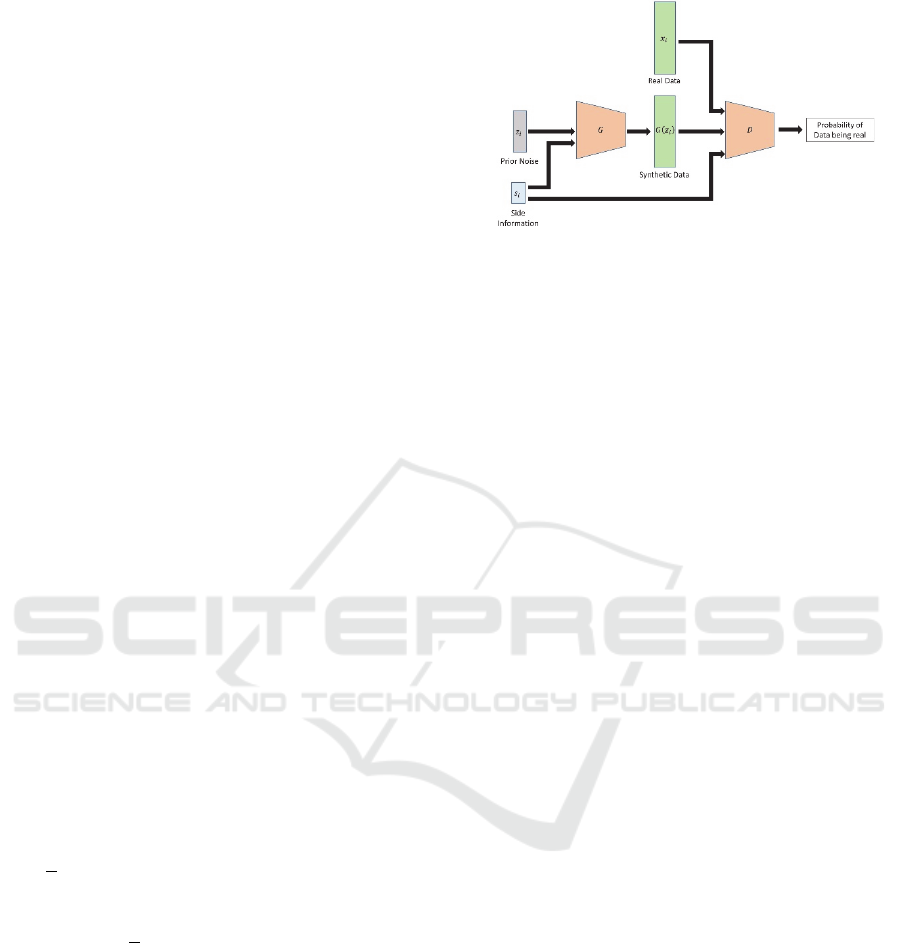
Figure 1: Visualization of the CGAN architecture. A set of

prior noise 𝑧



and side information 𝑠



corresponding to

sample 𝑥



are used to generate a synthetic sample. The

discriminator then uses the side information to predict if a

given sample is real or synthetic.

3 RESULTS

3.1 CGAN Training

CGAN models were trained only using the PRISM

dataset. Before training, microbial relative abundance

features present in less than 20% of samples or with a

mean abundance less than 0.1% across all samples of

both the PRISM and Validation sets were removed

from the analysis, resulting in a total of 93 microbial

features in the PRISM and Validation datasets.

In our analysis, we sample a vector of size 8 for

the input 𝑧



in the generator model. We add a vector

of size 2 representing the one-hot encoded value of

the disease state (IBD or healthy) as the input 𝑠



and

concatenate the two inputs together. The

concatenated input is then passed through two fully

connected layers of size 128. Batch normalization is

performed at each layer. The leaky ReLU activation

function with an alpha value of 0.1 is performed after

each batch normalization. Unlike the standard ReLU

activation function, leaky ReLU still allows a small

positive gradient for given negative values. The

output layer of the generator is a vector of size 93

representing the microbial features. The softmax

activation function in used in order to reconstruct the

relative abundance of the microbial community.

The discriminator network takes a vector of size

93 representing microbial relative abundance features

as an input in addition to vector of size 2 representing

the one-hot encoded disease state for that sample. The

two inputs are concatenated and fed through two fully

connected layers of size 128. The leaky ReLU

activation is again used for each fully connected

layer. The output of the discriminator is a single node

with a sigmoid activation to shrink the prediction

value to be between 0 and 1.

Using Conditional Generative Adversarial Networks to Boost the Performance of Machine Learning in Microbiome Datasets

105

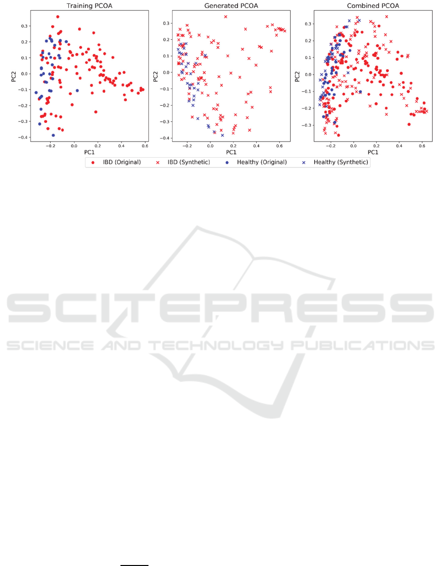
Figure 2: PCOA of the training (left), generated (middles), and combined (right) datasets using the Bray-Curtis dissimilarity.

Red points represent patients with IBD and blue points represent healthy subjects.

Models were trained using 10-fold cross-

validation. In each partition, 90% of the PRISM

dataset was used to train the CGAN model. CGAN

models were trained for 30,000 iterations in which 32

random samples were selected at each iteration as real

samples. A synthetic sample was generated for each

of the 32 real samples using the sample’s respective

disease state as the side information. The 32 real and

32 synthetic samples were then fed to the

discriminator for training and the discriminator was

updated based on Eq. 1. After updating the

discriminator, the discriminator is again used to

predict the synthetic samples and the generator is

updated based on Eq. 2. Both networks were trained

using the ADAM optimizer with a learning rate of

5x10

-5

(Kingma & Ba, 2014). For the implementation

and training of our CGAN models we used the

TensorFlow package in Python (Abadi et al., 2016).

During training, models were saved every 500

iterations. Additionally, the Principal Coordinate

Analysis (PCOA) (Wold, Esbensen, & Geladi, 1987)

of the training set, generated set, and the combination

of the two sets was visualized and stored. The Bray-

Curtis dissimilarity measure was used in calculating

the distance matrix for PCOA (Bray & Curtis, 1957).

The Bray-Curtis dissimilarity quantifies the microbial

compositional dissimilarity between two different

samples. Given two microbial samples, 𝑥



and 𝑥



the Bray-Curtis dissimilarity between the two

samples is calculated as

𝐵𝐶



𝑥



,𝑥





1

2𝐶



𝑆



𝑆



(3)

where 𝐶



is the sum of the lesser values for the

abundances of each species found in both 𝑥



and 𝑥



and 𝑆



and 𝑆



are the total number of species counted

in 𝑥



and 𝑥



respectively. Visual analysis of the

PCOA plots and the overlap of the original and

generated data was used to select the best model. An

example showing the PCOA of a selected model from

the cross-validated training is shown in Fig. 2.

3.2 Generated Data Improve

Prediction Performance

For each of the partitions in the 10-fold cross-

validation, we simulated 10,000 samples for both IBD

and healthy groups using the selected best model.

Relative abundance values were then log-transformed

and normalized to zero mean and unit variance. Next,

we trained logistic regression and multilayer

perceptron neural network (MLPNN) models to

predict disease status using microbial features. For

each partition of the cross-validation training, two

sets of MLPNN and logistic regression models were

trained. One set of models was trained using the

original samples in the partition of the training set.

The second set of models was trained using the

10,000 simulated samples generated by the CGAN

trained on the training set.

To train a logistic regression model on each 90%

used as training set, we performed internal 5-fold

cross-validation grid search over L1, L2, and Elastic

Net regularizations considering 10 penalty strengths

spaced evenly on a log scale ranging from 1 to 10,000.

Logistic regression models were trained using the

Python scikit-learn package (Pedregosa et al., 2011).

MLPNN models were trained using two fully

connected hidden layers with 256 nodes each and

dropout with a rate of 0.5 after each layer. Leaky

ReLU with an alpha of 0.1 was used as the activation

function. The output layer contained two nodes using

DeLTA 2020 - 1st International Conference on Deep Learning Theory and Applications

106

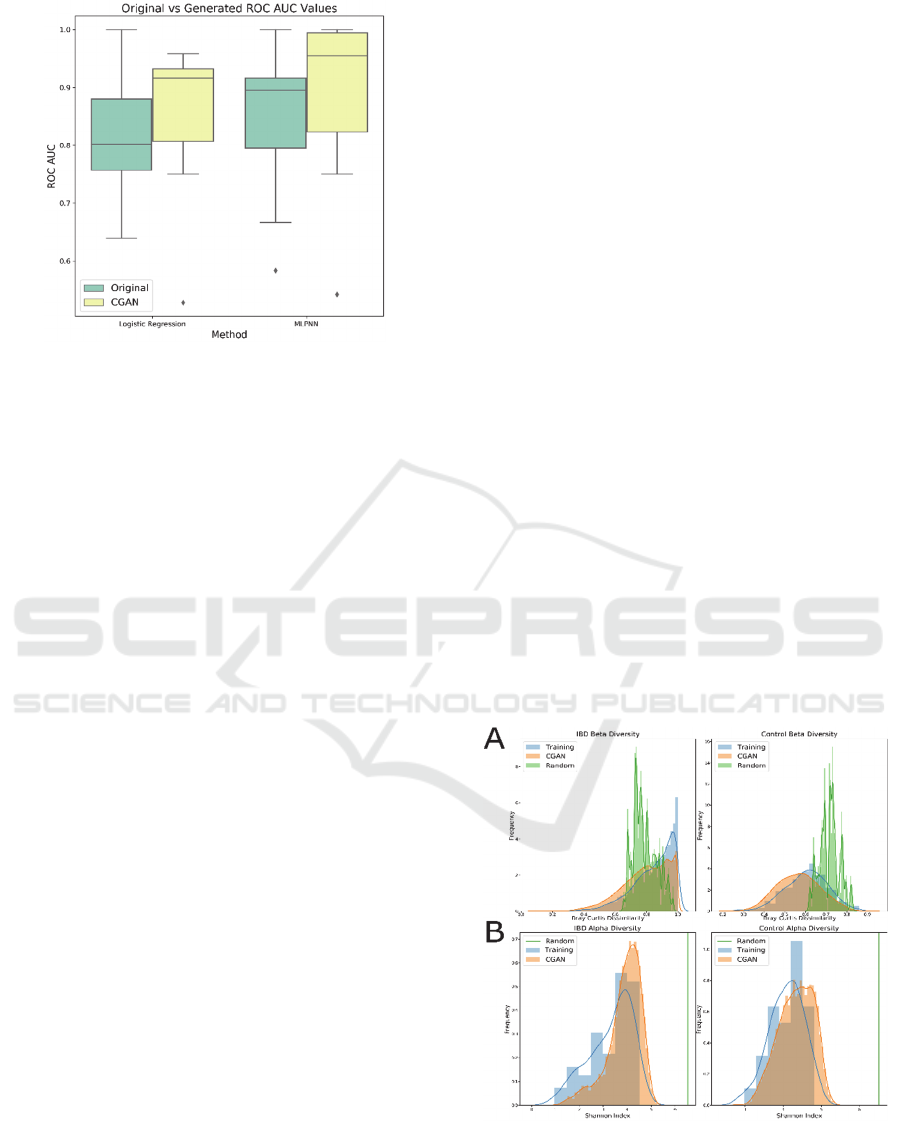
Figure 3: Boxplots for the ROC AUC values across 10-fold

cross-validation for logistic regression and MLPNN models

trained on original and synthetic data.

the softmax activation to predict the disease state.

Networks were trained using the ADAM optimizer

with a learning rate of 1x10

-4

. We set aside 20% of the

training set as a validation set and networks were

trained until the loss of the validation set had not

decreased for 100 epochs. The implementation and

training of the MLPNN models was again done using

the TensorFlow package in Python (Abadi et al., 2016).

Using the trained logistic regression and MLPNN

models generated from a fold’s training set as well as

the generated dataset, we calculated the area under the

receiver operating characteristic curve (ROC AUC)

using the fold’s 10% held out data of true observed

values. We observed that for logistic regression, the

models trained using the generated sets had an

average ROC AUC of 0.849 while the models trained

on the original data had an average ROC AUC of

0.778 across the 10 folds. Similarly, for MLPNN

models, the ROC AUC had a value of 0.889 when

training on the generated data and 0.847 when

training on the original data. Using a Wilcoxon

Signed-Rank test, the ROC AUC when using the

generated samples was significantly larger than that

of when using the original data with a p-value of

0.0249 for logistic regression models and a p-value of

0.0464 for MLPNN models. Boxplots of the ROC

AUC values when using original and generated

datasets is shown in Fig. 3. These results

demonstrated that the CGAN augmented datasets can

boost the predictive power of the ML models.

3.3 Diversity of Generated Data

Diversity metrics are often used to characterize

microbiome samples and datasets. In order to check

how well the generated samples represent the real

samples, we compare the distributions of the alpha

and beta diversities for IBD and healthy samples.

Alpha diversity is a local measure of species

diversity within a sample. It characterizes the

microbial richness of a community. For our analysis,

we use the Shannon Entropy metric to quantify the

alpha diversity of samples. Given a sample 𝑥 with 𝑚

relative abun-dance values, the Shannon Entropy is

calculated as

𝐻



𝑥



𝑥



log



𝑥









(4)

Beta diversity, on the other hand, allows us to

quantify how similar samples are to each other. In our

study, we use the Bray-Curtis dissimilarity as a

distance measure of beta diversity, calculated as

described in Eq. 3.

To demonstrate the behaviour of the CGAN

model, we visualize the diversity metrics for the

training set and for 10,000 generated samples using

the selected best model. In addition, we calculate the

diversity metrics of a set of 10,000 generated samples

using the random initialization of the CGAN before

any training to show the initial random distribution.

Before calculating the diversity metrics, we

clipped the generated samples in order to introduce

zero values. The softmax function used to generate

samples provides a vector entirely of positive values.

However, in reality microbiome data very sparse.

Figure 4: Distributions of (A) the beta diversity based on

the Bray-Curtis dissimilarity between the training set and

itself, the generated (CGAN), and random datasets, and (B)

the Shannon alpha diversity of training, generated, and

random samples for IBD (left) and healthy (right) samples.

Using Conditional Generative Adversarial Networks to Boost the Performance of Machine Learning in Microbiome Datasets

107

Therefore, to induce this sparsity into the

generated samples, we calculated the minimum value

across all species found in the training set. We used

this value as a threshold and set any generated value

less than the observed minimum to zero.

After clipping the generated sets, we calculated

the diversity metrics. When considering beta

diversity, we only considered the Bray-Curtis

dissimilarity from the training set to itself, the training

set to the best generated samples, and the training set

to the randomly generated samples. The distributions

of alpha and beta diversity for one of the cross-

validated partitions is shown in Fig. 4.

We observed that the data generated from the

selected best model followed very similar

distributions of the alpha and beta diversities of the

data used to train the CGAN. We did notice that the

beta diversity within the training set had a spike near

one, however upon post-analysis we discovered that

was caused by samples with only a few numbers of

microbial species present.

3.4 Generated Data Is Predictive of

External Dataset

To evaluate if the synthetic samples generated from

the CGAN model were generalizable to a dataset of a

similar study, we trained a CGAN model using the

entire PRISM dataset in the same manner as

described in Section 3.1. The CGAN is trained for

30,000 iterations and models as well as PCOA

visualization of the real and synthetic samples are

saved every 500 iterations. The best model is selected

based on the PCOA comparison between the training

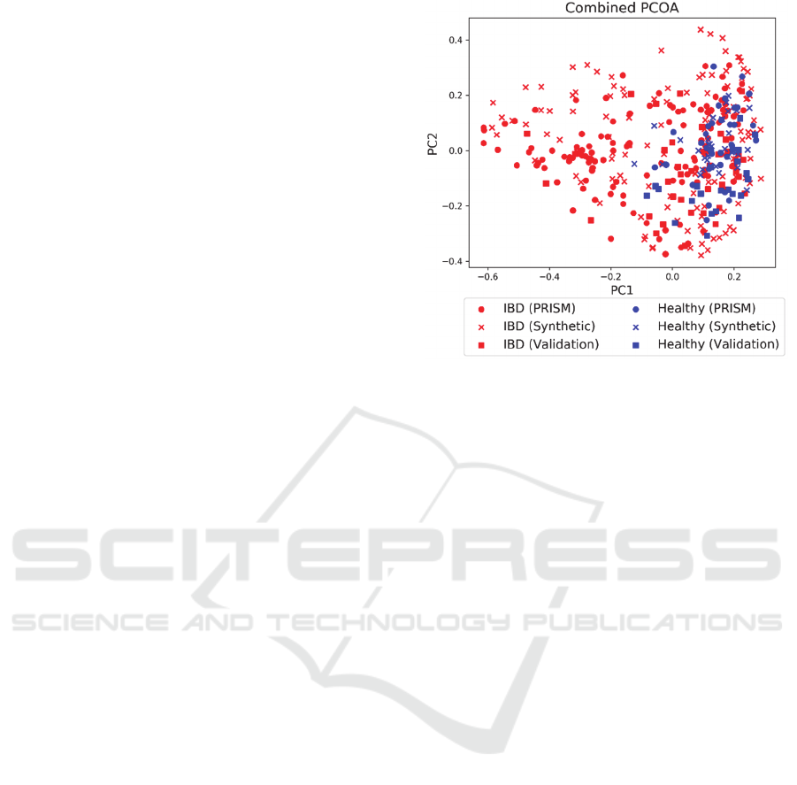
and generated sets. A PCOA visualization of the

PRISM dataset combined with the synthetic data

generated from the best model and the external

validation set is shown in Fig. 5.

Using the best model, we evaluate if the generated

samples can improve the task of predicting IBD

status. Logistic regression and MLPNN models are

trained in a similar fashion as outlined in Section 3.2.

The model was trained using 10,000 generated

samples from a CGAN model that was trained on the

entire PRISM dataset. We then evaluate the model

performance on the true observations of the external

validation IBD dataset. We observed an improvement

in ROC AUC from 0.734 to 0.832 in logistic

regression models and from 0.794 to 0.849 in

MLPNN models. This demonstrates that the synthetic

samples generated using one cohort can augment the

analysis of a different cohort.

Lastly, we analyse the distribution of alpha and

beta diversities of the original PRISM dataset, the

Figure 5: PCOA visualization of the combination of the

PRISM dataset, synthetic data generated by the best CGAN

model, and the external validation set. Red points represent

patients with IBD and blue points represent healthy

patients.

samples generated after training a CGAN on the

whole PRISM dataset, and the external validation

dataset. The alpha diversity is calculated for each

dataset using the Shannon Entropy metric. The beta

diversity within the PRISM dataset, from the PRISM

dataset to the generated samples, and from the

external validation dataset to the generated samples

was calculated. In addition, we compared the random

diversities from the randomly initialized CGAN

before training. The alpha and beta diversities are

shown in Fig. 6.

We observed that the beta diversity between the

PRISM dataset and the synthetic samples generated

from it displays similar distributions. Additionally,

the distribution of the beta diversity values between

the external validation set and the synthetic samples

follow a similar pattern, suggesting that the CGAN

model did not overfit the PRISM dataset and is robust

in generating synthetic samples. We also observed

that the alpha diversities within the PRISM, synthetic,

and external validation datasets showed similar

distributions. In particular, the alpha diversity within

the samples of IBD patients was very similar. The

distributions in the healthy samples were slightly

different in each of the datasets, however we suspect

this may be due to the fact that there were far fewer

cases of healthy samples in the original PRISM

dataset.

DeLTA 2020 - 1st International Conference on Deep Learning Theory and Applications

108

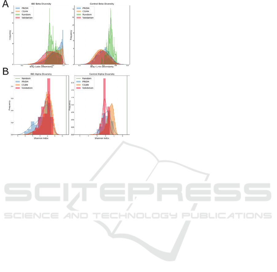
Figure 6: Distributions of (A) beta diversity based on the

Bray Curtis dissimilarity between the training set and itself,

the validation, the generated (CGAN), and random datasets

and (B) Shannon alpha diversity of training, validation,

generated, and random samples for IBD (left) and healthy

(right) samples.

4 CONCLUSIONS

In this study, we have developed a novel approach for

the generation of synthetic microbiome samples using

a CGAN architecture in order to augment ML

analyses. Using two different cohorts of subjects with

IBD, we have demonstrated that the synthetic

samples generated from the CGAN are similar to the

original data in both alpha and beta diversity metrics.

In addition, we have shown that augmenting the

training set by using a large number of synthetic

samples can improve the performance of logistic

regression and MLPNN in predicting host phenotype.

A current limitation to this approach involves

selecting the best CGAN model. Even though visual

inspection has been a common approach, it is a

subjective and may miss the optimal model. We plan

to further this study by investigating stopping criteria

using alpha and beta diversity metrics in order to

facilitate CGAN model selection. In addition, we plan

to evaluate other forms of side information such as

using time in longitudinal datasets.

REFERENCES

Abadi, M., Barham, P., Chen, J., Chen, Z., Davis, A., Dean,

J., Isard, M. (2016). Tensorflow: A system for large-

scale machine learning. Paper presented at the 12th

{USENIX} Symposium on Operating Systems Design

and Implementation ({OSDI} 16).

Barlow, G. M., Yu, A., & Mathur, R. (2015). Role of the

gut microbiome in obesity and diabetes mellitus.

Nutrition in clinical practice, 30(6), 787-797.

Bowles, C., Chen, L., Guerrero, R., Bentley, P., Gunn, R.,

Hammers, A., Rueckert, D. (2018). GAN

Augmentation: Augmenting Training Data using

Generative Adversarial Networks.

Bray, J. R., & Curtis, J. T. (1957). An Ordination of the

Upland Forest Communities of Southern Wisconsin.

Ecological Monographs, 27(4), 326-349.

doi:10.2307/1942268

Carabotti, M., Scirocco, A., Maselli, M. A., & Severi, C.

(2015). The gut-brain axis: interactions between enteric

microbiota, central and enteric nervous systems. Annals

of gastroenterology, 28(2), 203-209.

Che, Z., Cheng, Y., Zhai, S., Sun, Z., & Liu, Y. (2017, 18-

21 Nov. 2017). Boosting Deep Learning Risk

Prediction with Generative Adversarial Networks for

Electronic Health Records. Paper presented at the 2017

IEEE International Conference on Data Mining

(ICDM).

Franzosa, E. A., Sirota-Madi, A., Avila-Pacheco, J.,

Fornelos, N., Haiser, H. J., Reinker, S., Xavier, R. J.

(2019). Gut microbiome structure and metabolic

activity in inflammatory bowel disease. Nature

microbiology, 4(2), 293-305. doi:10.1038/s41564-018-

0306-4

Frid-Adar, M., Diamant, I., Klang, E., Amitai, M.,

Goldberger, J., & Greenspan, H. (2018). GAN-based

synthetic medical image augmentation for increased

CNN performance in liver lesion classification.

Neurocomputing, 321, 321-331.

Fung, T. C., Olson, C. A., & Hsiao, E. Y. (2017).

Interactions between the microbiota, immune and

nervous systems in health and disease. Nature

neuroscience, 20(2), 145.

Ghahramani, A., Watt, F. M., & Luscombe, N. M. (2018).

Generative adversarial networks simulate gene

expression and predict perturbations in single cells.

BioRxiv, 262501.

Goodfellow, I., Pouget-Abadie, J., Mirza, M., Xu, B.,

Warde-Farley, D., Ozair, S., Bengio, Y. (2014).

Generative adversarial nets. Paper presented at the

Advances in neural information processing systems.

Gopalakrishnan, V., Helmink, B. A., Spencer, C. N.,

Reuben, A., & Wargo, J. A. (2018). The influence of

the gut microbiome on cancer, immunity, and cancer

immunotherapy. Cancer cell, 33(4), 570-580.

Kingma, D., & Ba, J. (2014). Adam: A Method for

Stochastic Optimization. International Conference on

Learning Representations.

Knights, D., Parfrey, L. W., Zaneveld, J., Lozupone, C., &

Knight, R. (2011). Human-associated microbial

Using Conditional Generative Adversarial Networks to Boost the Performance of Machine Learning in Microbiome Datasets

109

signatures: examining their predictive value. Cell host

& microbe, 10(4), 292-296. doi:10.1016/j.chom.

2011.09.003

Kurilshikov, A., Wijmenga, C., Fu, J., & Zhernakova, A.

(2017). Host Genetics and Gut Microbiome: Challenges

and Perspectives. Trends in Immunology, 38(9), 633-

647. doi:https://doi.org/10.1016/j.it.2017.06.003

LaPierre, N., Ju, C. J. T., Zhou, G., & Wang, W. (2019).

MetaPheno: A critical evaluation of deep learning and

machine learning in metagenome-based disease

prediction. Methods. doi: https://doi.org/10.1016/

j.ymeth.2019.03.003

Mikołajczyk, A., & Grochowski, M. (2018, 9-12 May

2018). Data augmentation for improving deep learning

in image classification problem. Paper presented at the

2018 International Interdisciplinary PhD Workshop

(IIPhDW).

Mirza, M., & Osindero, S. (2014). Conditional generative

adversarial nets. arXiv preprint arXiv:1411.1784.

Pasolli, E., Truong, D. T., Malik, F., Waldron, L., & Segata,

N. (2016). Machine learning meta-analysis of large

metagenomic datasets: tools and biological insights.

PLOS Computational Biology, 12(7).

Pedregosa, F., Varoquaux, G., Gramfort, A., Michel, V.,

Thirion, B., Grisel, O., Duchesnay, É. (2011). Scikit-

learn: Machine Learning in Python. J. Mach. Learn.

Res., 12(null), 2825–2830.

Rong, R., Jiang, S., Xu, L., Xiao, G., Xie, Y., Liu, D. J.,

Zhan, X. (2019). MB-GAN: Microbiome Simulation

via Generative Adversarial Network. BioRxiv, 863977.

doi:10.1101/863977

Segata, N., Waldron, L., Ballarini, A., Narasimhan, V.,

Jousson, O., & Huttenhower, C. (2012). Metagenomic

microbial community profiling using unique clade-

specific marker genes. Nature Methods, 9(8), 811-814.

doi:10.1038/nmeth.2066

Tigchelaar, E. F., Zhernakova, A., Dekens, J. A. M.,

Hermes, G., Baranska, A., Mujagic, Z., Feskens, E. J.

M. (2015). Cohort profile: LifeLines DEEP, a

prospective, general population cohort study in the

northern Netherlands: study design and baseline

characteristics. BMJ open, 5(8), e006772-e006772.

doi:10.1136/bmjopen-2014-006772.

Tilg, H., & Kaser, A. (2011). Gut microbiome, obesity, and

metabolic dysfunction. The Journal of Clinical

Investigation, 121(6), 2126-2132.

Wold, S., Esbensen, K., & Geladi, P. (1987). Principal

component analysis. Chemometrics and intelligent

laboratory systems, 2(1-3), 37-52.

Xu, L., Paterson, A. D., Turpin, W., & Xu, W. (2015).

Assessment and Selection of Competing Models for

Zero-Inflated Microbiome Data. PloS one, 10(7),

e0129606-.doi:10.1371/journal.pone.0129606.

DeLTA 2020 - 1st International Conference on Deep Learning Theory and Applications

110