
Reliable Modeling for Safe Navigation of Intelligent Vehicles:
Analysis of First and Second Order Set-membership TTC
Nadhir Mansour Ben Lakhal
1,2
, Othman Nasri
2
, Lounis Adouane
3
and Jaleleddine Ben Hadj Slama
2
1
Institut Pascal, UCA/SIGMA - UMR CNRS 6602, Clermont Auvergne University, France
2
LATIS Lab, National Engineering School of Sousse (ENISo), University of Sousse, BP 264 Sousse Erriadh 1023, Tunisia
3
Heudiasyc UMR CNRS/UTC 7253, Université de Technologie de Compiègne, 60203 Compiègne, France
Keywords:
Intelligent Vehicles, Risk Management, Interval-based Modeling, Correlation Analysis, Interval Polynomial,
Second-order Time to Collision.
Abstract:
Developing high fidelity models to compute the Time-To-Collision (TTC) between vehicles is addressed in this
work. A TTC interval value is over-approximated while considering several uncertainties via interval analysis.
Furthermore, to decrease modeling inaccuracy, a novel second-order set-membership TTC formalization is
introduced by solving a polynomial equation with interval coefficients. This latter is derived from vehicles’
motion equations. Hence, an approach based on correlation analysis is exploited to improve the uncertainty
evaluation. The simulation results applied on an adaptive cruise control system of both high/low-order TTC
formalizations prove that the low-order model inaccuracy is compensated. Thanks to interval analysis and
correlation characterization, a great balance between modeling accuracy and simplicity is reached.
1 INTRODUCTION
Risk management should be inspected carefully to
employ autonomous vehicles in public roads (Nasri
et al., 2019). For the sake of safety, focus is currently
given to provide efficient solutions for in-road risk
identification. Thus, factors that stand behind the reli-
ability and accuracy of safety verification techniques
should be analyzed.
Advanced perception/communication devices and
navigation scene analysis have been used to capture
in-road hazards (Abdi and Meddeb, 2018), (Kasmi
et al., 2019). Nonetheless, these tools are prone to se-
vere uncertainties. To overcome uncertainty impacts,
several methods have been proposed in the literature
(Lakhal et al., 2019a), (Lozenguez et al., 2011). The
uncertainty is propagated into the navigation process
via stochastic models such as the Kalman filter, etc.
A specific probability distribution, as the Gaussian
function, is assumed to describe the uncertainty evo-
lution. This assumption is controversial, and changes
in noise features may occur (Rigatos, 2012). Addi-
tionally, most uncertainty evolution models are sen-
sitive to non-linearity (Wang et al., 2018). On top
of that, an accurate knowledge of the initial states of
the studied system is required, which is not evident
(Nicola and Jaulin, 2018). Hence, it is important to
study alternative approaches that are less sensitive to
these errors.
Otherwise, risk management reliability depends
on the accuracy of models used to derive numer-
ous risk indicators. For instance, the Time To Col-
lision (TTC) has been widely used for risk identifica-
tion (Iberraken et al., 2018), (Iberraken et al., 2019).
Tremendous attempts have been made to improve the
TTC precision. A comparative study between diverse
TTC formalizations could be found in (Hou et al.,
2014). A hidden Markov model has been used to pre-
dict the driving intention of nearby vehicles for more
accurate TTC estimation (Yang et al., 2020). Algo-
rithms computing distances between boxes bounding
vehicles were proposed to calculate TTC for com-
plex traffic scenarios (Wang et al., 2018). A vehicle
motion-based concept, named looming, was exploited
to decrease the TTC false alarms (Ward et al., 2015).
Interval analysis is a reliable way to handle uncer-
tainties/modeling imperfections (Jaulin et al., 2001).
It turns standard data to intervals to bound uncer-
tainty impacting the studied system (Moore et al.,
2009). Correspondingly, interval analysis may con-
tribute strongly in characterizing the uncertainty evo-
lution into intelligent transportation systems. In pre-
vious work, an interval-based model to compute TTC
for a car-following scenario was proposed to handle
Ben Lakhal, N., Nasri, O., Adouane, L. and Slama, J.
Reliable Modeling for Safe Navigation of Intelligent Vehicles: Analysis of First and Second Order Set-membership TTC.
DOI: 10.5220/0009890305450552
In Proceedings of the 17th International Conference on Informatics in Control, Automation and Robotics (ICINCO 2020), pages 545-552
ISBN: 978-989-758-442-8
Copyright
c
2020 by SCITEPRESS – Science and Technology Publications, Lda. All rights reserved
545

uncertainties and communication latencies (Lakhal
et al., 2019b) and (Lakhal et al., 2019c). Moreover,
the interval TTC over-approximation was optimized
via a data-driven characterization of correlation that
would relate the navigation system variables. In this
paper, we build on this previous work to analyze
much comprehensively the performances of the set-
membership modeling. The main contribution of this
work is to introduce a novel second-order interval-
based TTC over-approximation to consider more pa-
rameters intervening in the car-following scenario.
The high-order model consists in a quadratic poly-
nomial with interval coefficients generated from ve-
hicles’ motion equations. Usually dedicated to bound
the rounding errors, interval polynomials have never
been used to build models for uncertainty evolution
into navigation systems. Afterwards, simulation is
elaborated on an Adaptive Cruise Control (ACC). The
performances of the interval high and low-order TTC
in conducting the risk worst-case analysis are com-
pared. The quality of the set-membership modeling
joined with the correlation analysis is evaluated in
terms of accuracy and simplicity.
The rest of this paper is arranged as follows:
Section 2 introduces the first and second-order TTC
interval-based formalizations. Section 3 presents an
algorithm to find roots for an interval polynomial to
approximate the TTC. Section 4 explains the correla-
tion analysis role in ameliorating the findings of the
TTC set-membership models. Section 5 presents the
simulation results. Section 6 concludes the results of
this work and discusses some future work.
2 SECOND ORDER
SET-MEMBERSHIP TTC
For a car-following scenario, the TTC is often ap-
proximated by the ratio between the distance separat-
ing two vehicles and their relative velocity. Instead,
the evolution of the spacing distance between the fol-
lower and the leader is used in this paper to perform
more accurate collision prediction. In this way, all the
interactions between vehicles are taken into account.
Let consider two vehicles i and j, which are respec-
tively the leader and the follower. V
i
, V
j
, p
i
and p
j
are
their respective velocities and vector positions. Ac-
cording to (Ward et al., 2015), the separation evolu-
tion between both vehicles is described at each instant
by:
• The separation distance:
d
i j
=
q
(p
i
− p
j
)
T
(p
i
− p
j
) (1)
• The change rate in the separation distance:
˙
d
i j
=
1
d
i j
(p
i
− p
j
)
T
(V
i
−V
j
) (2)
• The variation of the change rate in the separation
distance is governed by the following equation:
¨
d
i j
=
1
d
i j
(V
i
−V
j
)
T
(V
i
−V
j
) −
˙
d
2
i j
(3)
Equations (2) and (3) are obtained by the consecutive
differentiation of equation (1). In practice, d
i j
is mea-
sured in run-time thanks to diverse vehicular tools as
a LiDAR or laser scanner. Therefore, the authors in
(Ward et al., 2015) defined T TC
1
as a first order TTC:
T TC
1
= −
d
i j
˙
d
i j
(4)
However, equation (4) neglects parameter
¨
d
i j
. Model
simplification is the main source of errors (Khelifi
et al., 2018). In an effort to improve accuracy, the au-
thors in (Ward et al., 2015) upgraded the TTC approx-
imation to a second-order expression. When
¨
d
i j
6= 0,
a second-order TTC, denoted T TC
2
, is obtained by
solving the following polynomial:
d
i j
+
˙
d
i j
T TC
2
+
1
2
¨
d
i j
T TC
2
2
= 0 (5)
Note that equation (5) is derived from the vehicles’
motion equations. The polynomial roots underline at
which instants the two vehicles collide, and the sepa-
ration between them is zero. Accordingly, the authors
in (Ward et al., 2015) defined the T TC
2
value depend-
ing on the roots of equation (5). When
¨
d
i j
= 0 or the
polynomial has no real roots, the low-order model is
used and T TC
2
= T TC
1
. In the case of two real posi-
tive roots, the lower value is attributed to T TC
2
since
it presents the first collision time. If one of the roots
is positive and the other is negative, the positive one
is taken. Both roots can be also negative. In such a
situation, the root with the closest absolute value to
zero is selected because it consists of the most recent
interaction between the motions of both vehicles.
Despite its accuracy, the high-order TTC is still
sensitive to uncertainty and communication latencies.
To overcome this issue, interval analysis is adopted
in this paper. Data representation is extended to
intervals. Mathematical operations (+, −,∗,/) and
functions (sin, cos, etc.) are extended to handle inter-
vals (Jaulin et al., 2001). Subsequently, the obtained
interval-based models provide over-approximations
of results that definitely enclose the exact outputs.
Henceforth, [x] = [x,x] is a real interval, where x and
x are its lower and upper bounds. The width of [x]
ICINCO 2020 - 17th International Conference on Informatics in Control, Automation and Robotics
546

underlines the uncertainty extent. Accordingly, equa-
tions (4) and (5) are represented as:
[T TC
1
] = −
[d
i j
]
[
˙
d
i j
]
(6)
[d
i j
] + [
˙
d
i j
][T TC
2
] +
1
2
[
¨
d
i j
][T TC
2
]
2
= 0 (7)
Since it describes the real behavior, the second-order
set-membership TTC is expected to be more accurate
than the first-order one. Equation (7) is a quadratic
polynomial with perturbed coefficients. Its roots are
intervals enclosing the collision exact time. Solving
this polynomial is not feasible by standard analyti-
cal approaches. A specific interval polynomial solver
must be used. Before doing so, a methodological
manner to quantify uncertainties attributed to each in-
terval measurement is introduced. The environmen-
tal circumstances, where more uncertainties are ex-
pected, are examined. At first, the following assump-
tions, which are based on the confidence intervals of
sensors and communication devices, are admitted:
• The localization inaccuracy is assessed via a sig-
nal strength indicator that considers the signal at-
tenuation in the navigation zone.
• The accumulated error impacting the separation
distance measurement is considered by an uncer-
tainty range of ±1% from the measured d
i j
.
• The follower speed V
j
is assumed to be exact, and
no uncertainty is attributed to this parameter.
• The leader speed V
i
is assumed to be erroneous
with a range of ±0.5% due to measurement im-
precision.
Afterwards, several latencies can slow down the auto-
motive system operation and prohibit the quick man-
agement of risks. For that reason, it is advisable to
consider such latencies by [T TC]. In this work, the
follower car is expected to receive the V
i
value via
a Vehicle-to-Vehicle (V2V) communication. Hence-
forth, latencies impacting the V2V communication
are characterized through interval [T
V 2V
]. The un-
certainty attributed to [T
V 2V
] is appraised through
the empirical research work depicted in (Dey et al.,
2016). Min/max values of latencies that may happen
were provided in (Dey et al., 2016). These bounds
were presented as a function of the vehicle speed and
the number of connected vehicles in close proximity
(communication conflicts increase delays). Besides,
[T
L
] is a constant interval that takes into account laten-
cies due to update time of sensors and the data prop-
agation into the embedded system. Consequently, the
TTC set-membership formalization must consider ex-
plicitly the aforementioned uncertainty sources:
[T TC
1
] = −
[d
i j
]
[
˙
d
i j
]
− [T
V 2V
] − [T
L
] (8)
[T TC
2
] = [ℜ] − [T
V 2V
] − [T
L
] (9)
where [ℜ] is the polynomial root of equation (7). Sim-
ilar to the deterministic case detailed above (cf. equa-
tion (5)), [ℜ] is the root corresponding to the first col-
lision time. Figure 1 illustrates the main instructions
of the proposed uncertainty quantification strategy to
over-approximate the first/second order TTC.
Figure 1: Interval-based risk management.
3 SOLVING QUADRATIC
INTERVAL POLYNOMIAL
Finding roots for interval polynomials has been
widely discussed in the literature. Several numerical
branch and bound algorithms were introduced for this
aim (Fan et al., 2008). Despite their accuracy, the cal-
culation time of these approaches was unpredictable.
One more category of approaches used polynomial
factorization and cumbersome mathematical calcula-
tion as an inverting interval matrix (Zhang and Deng,
2013). Other fast methods were developed (Ferreira
et al., 2001). Nevertheless, these approaches provided
just a prior estimate for the space containing the real
roots. In this work, real roots with sharp bounds of
interval polynomials are obtained by studying the in-
terval polynomial boundary functions.
Let consider a quadratic polynomial with the fol-
lowing shape:
P([x]) = [a]x
2
+ [b]x + [c] (10)
Intuitively, P([x]) can be expressed within its bound-
ary functions, where: P([x]) = [P([x]),P([x])]. For
such a polynomial, P([x]) and P([x]) may be derived
through all possible combinations between the coef-
ficient bounds. Indeed, eight real single-valued poly-
nomials are given from these combinations:
f
1
= ax
2
+ bx + c; f
2
= ax
2
+ bx + c
f
3
= ax
2
+ bx + c; f
4
= ax
2
+ bx + c
f
5
= ax
2
+ bx + c; f
6
= ax
2
+ bx + c
f
7
= ax
2
+ bx + c; f
8
= ax
2
+ bx + c
(11)
Reliable Modeling for Safe Navigation of Intelligent Vehicles: Analysis of First and Second Order Set-membership TTC
547
By interpreting the dominant term of P([x]), it is ev-
ident that P([x]) and P([x]) are respectively enclosed
between ( f
1
, f
2
, f
3
, f
4
) and ( f
5
, f
6
, f
7
, f
8
). It is clear
also that:
f
1
≤ f
2
; f
3
≤ f
4
f
6
≥ f
5
; f
7
≥ f
8
(12)
Subsequently, we can figure out that:
P(x) =
(
P
1
= ax
2
+ bx + c, if x ≥ 0
P
2
= ax
2
+ bx + c, if x ≤ 0
(13)
and
P(x) =
(
P
3
= ax
2
+
bx + c, if x ≥ 0
P
4
= ax
2
+ bx + c, if x ≤ 0
(14)
Note that P
i=1..4
= (P
1
, P
2
, P
3
, P
4
) represents non-
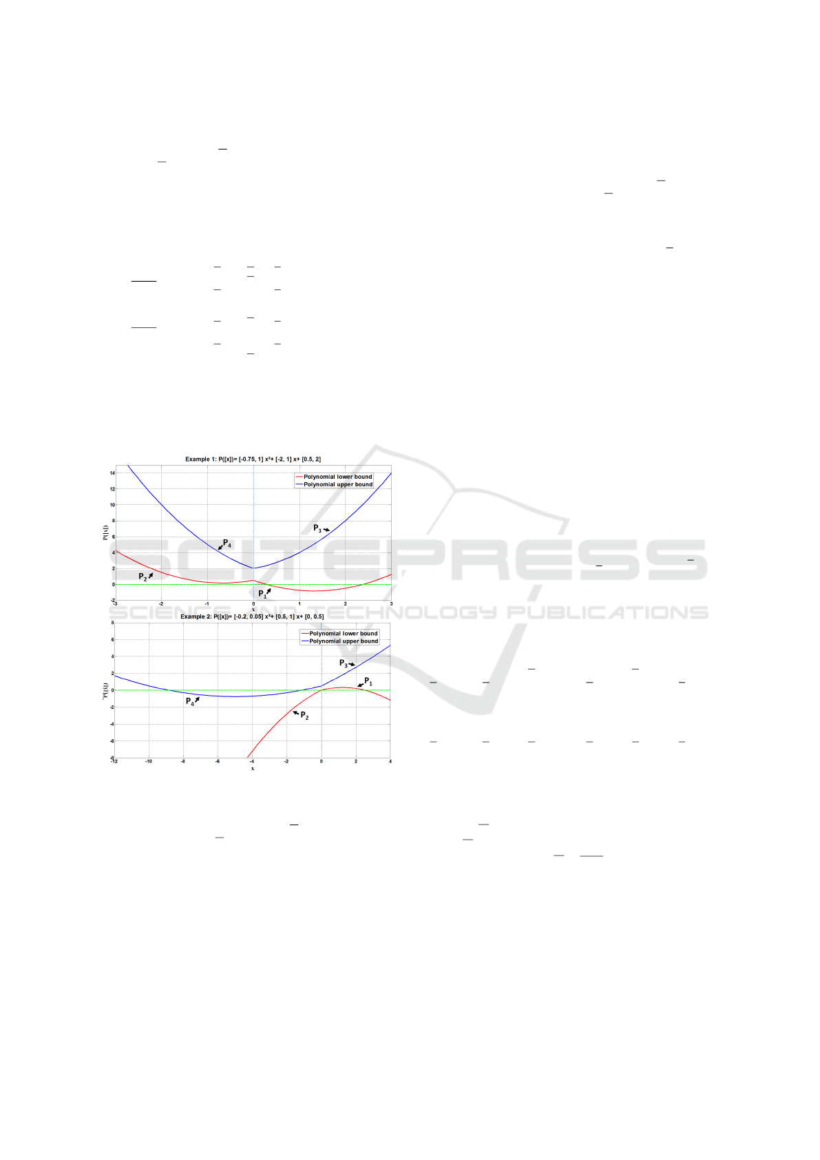
interval real boundary functions associated to P([x]).
To illustrate such a notion, Figure 2 presents two ex-
amples of quadratic polynomials with perturbed coef-
ficients.
Figure 2: Examples of interval polynomials.
An efficient way to find polynomial roots is to de-
termine sets where: P([x]) ≤ 0 ≤ P([x]). Eventually,
estimating sharp bounds of this intersection should be
accomplished by solving P
i=1..4
. Once the roots of the
boundary functions P
i=1..4
are calculated, it remains
to clarify how to join these roots to formulate a pre-
cise enclosure of P([x]) solutions. Contrary to non-
interval polynomials, P([x]) may have at maximum
three distinct interval roots, including semi-infinite in-
tervals (see Figure 2).
In this work, a simple algorithm is presented to ex-
tract P([x]) interval roots using P
i=1..4
. It is based on
the theoretical results obtained in (Hansen and Wal-
ster, 2002) and (Hansen and Walster, 2003), where
the P([x]) coefficient bounds are analyzed to figure
out the shape and orientation of P(x) and P(x). Con-
sequently, the right number and values of the interval
roots are appropriately determined.
First, the number of subcases that must be checked
to resolve P([x]) is decreased by admitting a > 0. In
the opposite case, the sign of P([x]) must be simply
reversed. Therefore, each P
i
must be solved by inter-
val arithmetic. The readers must distinguish between
solving interval polynomials and isolating real roots
of standard polynomials. Several set-membership al-
gorithms resolve the non-interval polynomials in or-
der to bound rounding errors.
In this work, the real roots of P
i=1..4
are computed
numerically via a specific interval computation pack-
age. The isolated real roots associated to each P
i
, in-
cluding multiple roots, are added to list L. Since func-
tions P
1
and P
2
bound P([x]) only for x ≥ 0 (see equa-
tion (13)), any negative root or part of a root must
indefinitely be discarded from L. Seemingly, posi-
tive roots or parts of roots associated to P
3
and P
4
are
dropped.
Otherwise, there are some particular cases that
must be considered while arranging L. Indeed, a dou-
ble root is obtained at x = 0 for (P
1
,P
2
) when c = 0
and respectively for (P
3
,P
4
) if c = 0. For both cases,
this root must be entered just one time into the list.
Besides, the infinite interval endpoints ±∞ must be
placed if necessary in L. Referring to (Hansen and
Walster, 2003), once the following cases are satisfied,
a lower endpoint −∞ is added to L :
a < 0 ∨ (a = 0 ∧ b > 0) ∨ (a = 0 ∧ b = 0 ∧ c ≤ 0)
(15)
Likewise, +∞ is added to L only if:
a < 0 ∨ (a = 0 ∧ b > 0) ∨ (a = 0 ∧ b = 0 ∧ c ≤ 0)
(16)
At this stage, L contains intervals that certainly
present a lower or upper end-point of the final inter-
val roots of P([x]). Thus, it is necessary to recog-
nize which are the lower and upper ones. Let denote
[S
i
] = [S
i
,S
i
] the set of intervals held in L. All intervals
[S
i
] are sorted such that S
i
≤ S
i+1
. It is worth mention-
ing that the adopted algorithm requires to consider
±∞ as degenerate intervals. Hence, n denotes the
number of intervals included in L (no more than six
roots 0 ≤ n ≤ 6). The final step from the root finding
strategy consists in arranging the solution according
to the obtained n. Table 1 summarizes all probable
shapes of the interval roots associated to P([x]). Fi-
nally, all necessary steps to solve the interval polyno-
mial are recapitulated in Algorithm 1.
ICINCO 2020 - 17th International Conference on Informatics in Control, Automation and Robotics
548
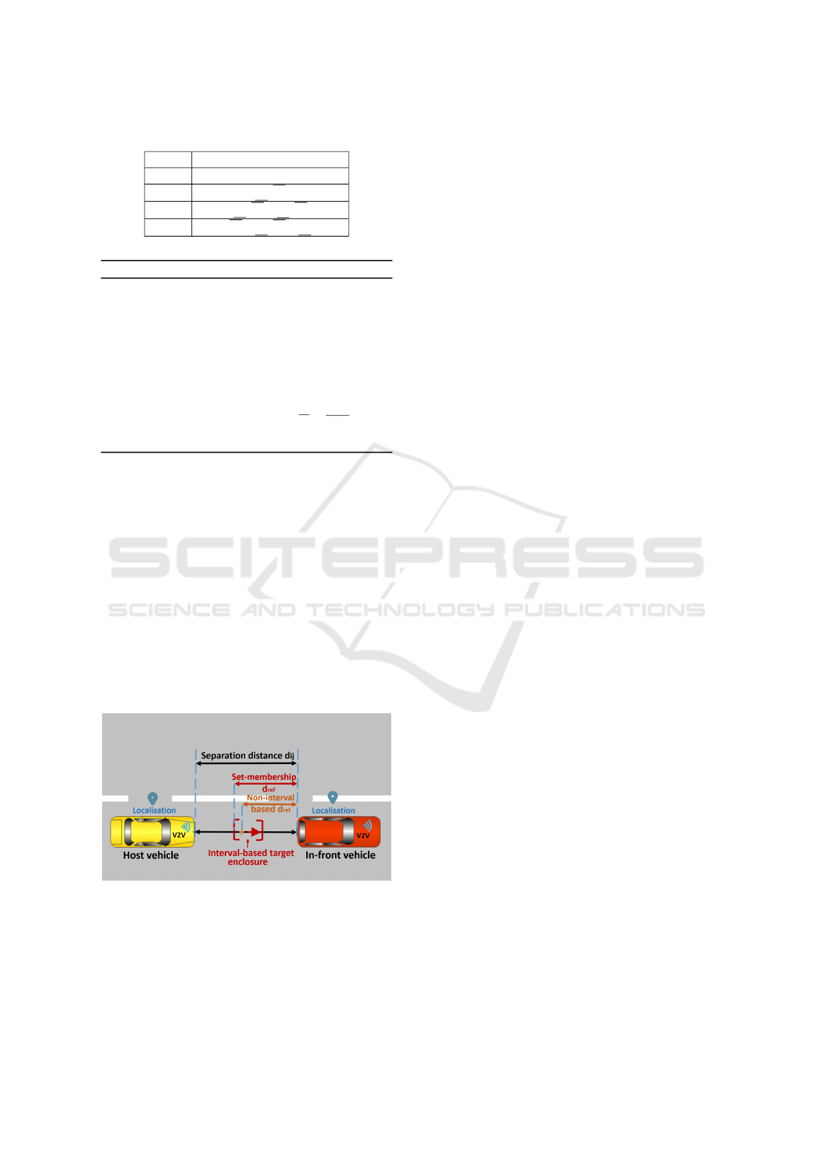
Table 1: Interval roots according to n.
Interval roots
n = 0 ∅
n = 2 [S
1
,S
2
]
n = 4 [S
1
,S
2
],[S
3
,S
4
]
n = 6 [−∞,S
2
],[S
3
,S
4
],[S
5
,+∞]
Algorithm 1: Solving Interval Polynomial.
Require: [a], [b] and [c]
Ensure : Solve P([x]) = [a]x
2
+ [b]x + [c]
1 -Define P
i=1..4
(cf. equations (12) and (13)).
2 -Find interval roots of P
i=1..4
.
3 -Put results in L.
4 -Add infinite entries ±∞ to L, if needed (cf.
equations (15) and (16)).
5 -Sort the interval elements in L (S
i
≤ S
i+1
).
6 -Check the length of L to define roots of
P([x]).
4 CORRELATION-BASED
OPTIMIZATION STEP
In this work, the interval-based TTC formalizations
are dedicated to ensure safety for a modern ACC sys-
tem. At every sample time, an interval enclosure for
the position of target assigned to the ACC-equipped
vehicle (follower) is defined proportionally to the cur-
rent [T TC], which is calculated via the first or second-
order formalization. Then, a reference distance, de-
noted d
re f
, is maintained from the in-front vehicle ac-
cording to the worst-case risk indicated by the target
enclosure (cf. Figure 3).
Figure 3: Proposed ACC risk management principle.
Nevertheless, the interval over-approximations ob-
tained through assumptions defined in section 2 are
too conservative. The occurrence of the worst cases of
uncertainties for all parameters considered in the TTC
computation is quite unrealistic. The main task of
ACC systems is to optimize the distance between ve-
hicles to prevent congestion and traffic disturbances.
In this sense, the model developed for risk identifica-
tion must make a trade off between safety and accu-
racy. As an enhancement for the interval-based mod-
els, a data-driven optimization step was introduced in
the previous work of (Lakhal et al., 2019b), (Lakhal
et al., 2019c) and (Ben Lakhel et al., 2016). Accord-
ingly, this approach is joined to the TTC second-order
model to obtain more compact bounds of findings.
In this section, the proposed data-driven optimization
approach is briefly recalled.
Correlation is a relevant statistical parameter to
describe the operation of systems. More focus is
given currently to correlation analysis to study the
performances of autonomous vehicles (Wu et al.,
2020). The main idea behind the proposed data-
driven-optimization step is to examine the correlation
progression over time. During the navigation run-
time, substantial and brutal changes in vehicle dy-
namics are unrealistic in few sampling periods. Based
on this understanding, the evolution of the correlation
states should be smooth. Only uncertainties and erro-
neous measurements may invoke an irregular progres-
sion of correlation. Various data-driven approaches
have relied on this assumption to capture faults or to
regress outliers (Xia et al., 2017), (Chen et al., 2019).
Uncertainties assigned to interval measurements
can be over-estimated. This fact may entail a brutal
variation in the correlation progression between two
successive instants: t
k−1
and t
k
. Hence, the proposed
approach narrows recursively intervals until obtaining
an acceptable progression in the correlation between
variables. Narrowing is interpreted once the corre-
lation relating the new tightened intervals matches
reference values characterized off-line. Let denote
by C
([X],[Y ])|k
the correlation relating interval variables
[X] and [Y ] at instant t
k
. The overall process to esti-
mate the correlation values for interval variables is de-
tailed in (Lakhal et al., 2019b). Thereafter, the gap in
the correlation between instants t
k
and t
k−1
, denoted
γ
k|k−1
, is estimated through equation (17):
γ
k|k−1
= C
([X],[Y ])|k
−C
([X],[Y ])|k−1
(17)
Interval widths must be narrowed in a recursive way
to adapt the value of γ
k|k−1
in run-time and elimi-
nate over-estimated uncertainties. For each couple of
interval-valued variables intervening in the TTC com-
putation, the interval with the largest width is con-
cerned with iterative narrowing. After that, narrowing
is aborted at two conditions:
• Condition 1. When γ
k|k−1
decreases from one
iteration to another and suddenly starts to raise;
i.e., the interval is narrowed as much as possible.
Reliable Modeling for Safe Navigation of Intelligent Vehicles: Analysis of First and Second Order Set-membership TTC
549
Extra-narrowing may cause an undesirable modi-
fication in the correlation structure.
• Condition 2. Once γ
k|k−1
exceeds the minimum
variation of correlation, which is recorded during
the off-line simulation of a normal system opera-
tion.
Algorithm 2: [TTC] Optimized Estimation.
Input : p
i
, p
j
, V
i
, V
j
, d
i, j
,[T
V 2V
] and [T
L
].
Output: [T TC
1
] and [T TC
2
].
1 while Navigation process is running do
2 -Define [d
i, j
], [
˙
d
i j
], [
¨
d
i j
], [V
i
], [p
i
] and [p
j
].
3 for each couple of variables between
instants t
k
and t
k−1
do
4 repeat
5 -Calculate C
([X],[Y ])|k
.
6 -Estimate γ
k|k−1
(equation (17)).
7 -Narrow the interval, if needed.
8 until Condition 1 or 2 is satisfied
9 end
10 -Evaluate [T TC
1
] and [T TC
2
] (see
equations (10) and (11))
11 end
5 SIMULATION RESULTS
In this section, the reliability of the proposed interval-
based models to compute the TTC is demonstrated.
The quantitative results obtained from the conducted
simulation are analyzed to provide a qualitative com-
parison between the performances of the first-order
and second-order TTC formalizations.
5.1 Test Scenario and Simulation Setups
The overall set-membership TTC-based risk manage-
ment is tested under a MATLAB freeway naviga-
tion simulator. Vehicle motions implicated in the test
phase are simulated through the well-known tricycle
kinematic model. The elaborated test scenario con-
sists of a car-following scenario in a highway road.
In addition, a model of a highway-road segment is
selected as the test-scene. Otherwise, a white Gaus-
sian noise is injected in the exact measurements of the
navigation dynamics during simulation.
As already said, the follower vehicle is equipped
with an ACC system. This latter exploits bounds of
the interval TTC (according to the first or second-
order model) to take precaution of the risk worst cases
and adapt the reference distance from the vehicle
ahead. Full details about the ACC operation princi-
ple are available in (Lakhal et al., 2019c).
Technically speaking, the interval computation is
ensured by the reliable computation package INT-
LAB (Rump, 1999). All the simulation work depicted
in this section is carried out under MATLAB on an
Intel i5 Processor with 3.5 GHz and 16 GB memory.
More configurations involved in the established sim-
ulation are recapitulated in Table 2.
Table 2: Simulation setups.
Parameter Value
Sampling step 0.1 (s)
Sensors update time 0.01 (s)
Follower embedded system delay 0.025 (s)
Leader maximum velocity 22 (m/s)
Follower maximum velocity 23 (m/s)
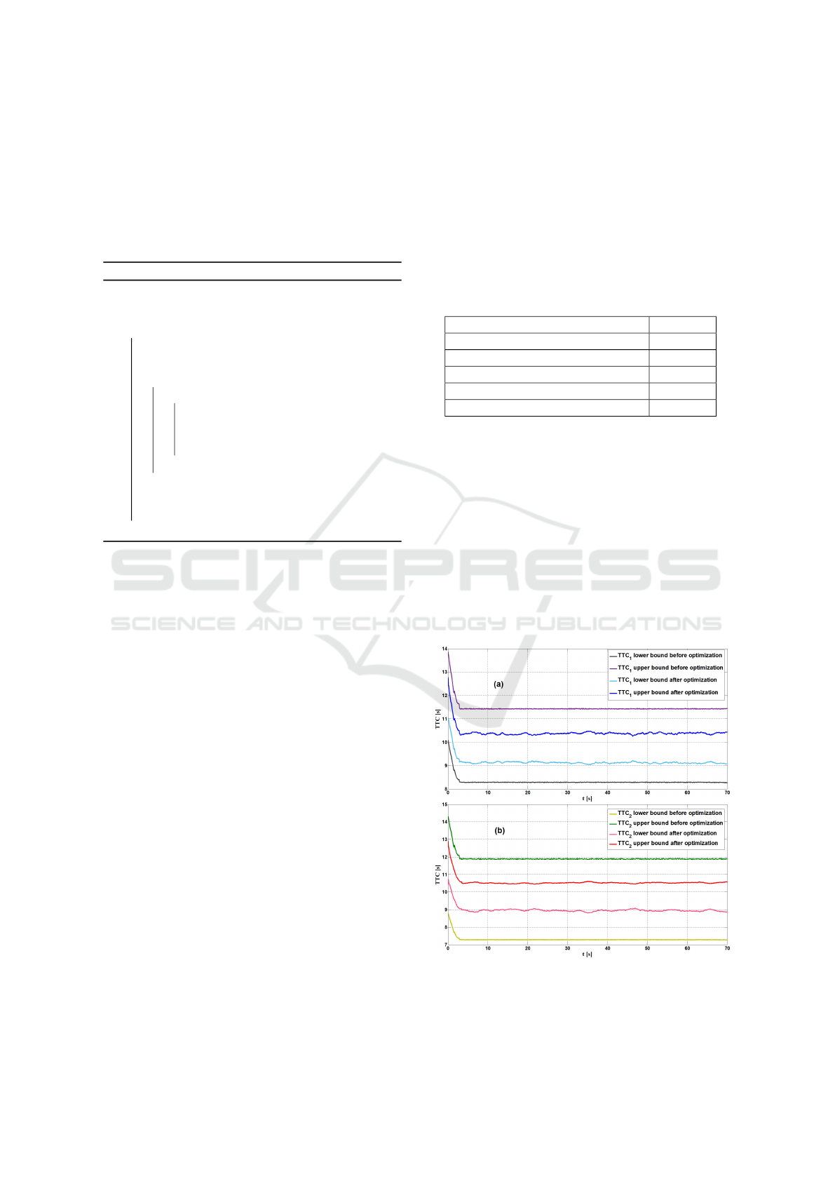
5.2 Results and Discussion
At first, the role of the correlation analysis in provid-
ing more sharp bounds of TTC values is inspected.
As shown in Figure 4, the TTC enclosures are effi-
ciently narrowed for both [T TC
1
] and [T TC
2
]. For
the first-order set-membership formalization, initial
amounts of uncertainties are minimized with an aver-
age range of 60.3%. Similarly, the average reduction
in the width of [T TC
2
] due to the correlation-based
optimization step is about 65.79%.
Figure 4: T TC
1
and T TC
2
enclosures with/without opti-
mization step.
ICINCO 2020 - 17th International Conference on Informatics in Control, Automation and Robotics
550
More importantly, the results of the interval high-
order TTC computation model are more conservative
than the low-order one. In average, the widths of
[T TC
1
] and [T TC
2
] are respectively about 1.25s and
1.579s. This fact can be explained by the “depen-
dency effect" characterizing the interval arithmetic
(Moore et al., 2009). Indeed, variables occurring sev-
eral times in one expression are assumed as indepen-
dently varying over their enclosures, which may lead
to an additional pessimism in the results. Hence, more
pessimism is entailed by upgrading the first-order-
model to a second-order formalization since the num-
ber of the involved variables is increased.
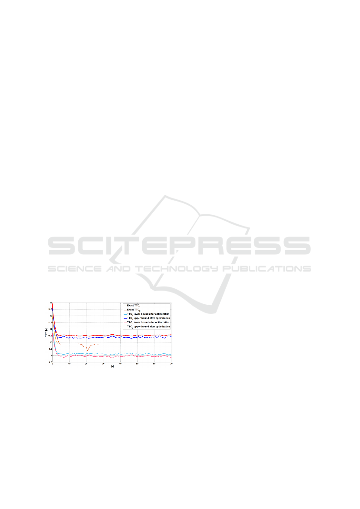
In a second place, Figure 5 illustrates the evolution
of the exact T TC
1
and T TC
2
. These exact values of
T TC
1
and T TC
2
are obtained in a deterministic way
(respectively via equations (4) and (5)) without any
noise injection during the simulation. All along the
simulation run-time, the results of the two developed
interval-based formalizations of the TTC enclose per-
fectly the reference values provided by the exact evo-
lution of T TC
1
and T TC
2
. Correspondingly, the con-
sistency of the set-membership modeling joined with
the correlation analysis is proven. Even more, the
first-order interval-based TTC is more accurate than
the second-one since it provides sharp bounds and si-
multaneously encompasses the exact and real values
of the TTC. This fact optimizes implicitly the naviga-
tion traffic flow because it decreases the reference dis-
tance maintained between vehicles. Eventually, the
interval-based uncertainty quantification method con-
tributes to compensate the inaccuracy presented by
the first-order TTC resulting from the modeling sim-
plification.
Figure 5: T TC
1
and T TC
2
enclosures compared with exact
results.
Another advantage of the proposed approach is the
reduction in the computational cost of the risk man-
agement of intelligent vehicles. Using simple mod-
els, which handle efficiently all possible uncertainties,
helps to respect the real-time constraints. In our case
of study, solving the interval quadratic polynomial to
compute an over-approximation to the TTC requires
0.09s as an average execution time. Therefore, the
T TC
1
is more efficient as a risk indicator than the
T TC
2
especially in terms of computational demands.
Additionally, the accuracy-level ensured by the T TC
1
is sufficient to guarantee the navigation safety since it
handles properly uncertainties and modeling errors.
6 CONCLUSIONS
The reliability of models employed for the risk man-
agement of intelligent navigation systems is of ut-
most importance. In this work, first and second-order
interval-based models to compute the TTC between
two vehicles are introduced. Set-membership mod-
eling allows considering various uncertainties and la-
tencies that can emphasize collision risks. Moreover,
the evolution of the correlation that relates variables
is characterized to improve the uncertainty evalua-
tion. Then, the performances of both proposed mod-
els are compared. The results of the first-order TTC
are more compact and permit handling efficiently all
uncertainties. Fast risk analysis with the same accu-
racy level of the second-order TTC is ensured via the
simple low-order model. A trade off between accu-
racy and simplicity is ensured by joining the interval-
based computation with correlation analysis. Accord-
ingly, the need for sophisticated models for intelligent
vehicles’ motions to make the risk management suc-
cessful is discarded, while mastering all uncertainty-
induced risks.
Otherwise, the proposed method should be inte-
grated in the future on a real vehicle and applied for
more critical maneuvers such as lane changes.
ACKNOWLEDGEMENTS
The present work is supported by the WOW (Wide
Open to the World) program of the CAP 20-25
project. It receives also the support of IMobS3 Labo-
ratory of Excellence (ANR-10-LABX-16-01).
REFERENCES
Abdi, L. and Meddeb, A. (2018). Driver information sys-
tem: a combination of augmented reality, deep learn-
ing and vehicular ad-hoc networks. Multimedia Tools
and Applications, 77(12):14673–14703.
Ben Lakhel, N. M., Nasri, O., Gueddi, I., and Ben Hadj
Slama, J. (2016). Sdk decentralized diagnosis with
vertices principle component analysis. In 2016 Inter-
national Conference on Control, Decision and Infor-
mation Technologies (CoDIT), pages 517–522.
Reliable Modeling for Safe Navigation of Intelligent Vehicles: Analysis of First and Second Order Set-membership TTC
551

Chen, L., Yang, X., Liu, P. X., and Li, C. (2019). A novel
outlier immune multipath fingerprinting model for in-
door single-site localization. IEEE Access, 7:21971–
21980.
Dey, K. C., Rayamajhi, A., Chowdhury, M., Bhavsar,
P., and Martin, J. (2016). Vehicle-to-vehicle (v2v)
and vehicle-to-infrastructure (v2i) communication in
a heterogeneous wireless network – performance eval-
uation. Transportation Research Part C: Emerging
Technologies, 68:168–184.
Fan, X., Deng, J., and Chen, F. (2008). Zeros of univariate
interval polynomials. Journal of Computational and
Applied Mathematics, 216(2):563–573.
Ferreira, J., Patrıcio, F., and Oliveira, F. (2001). A pri-
ori estimates for the zeros of interval polynomials.
Journal of Computational and Applied Mathematics,
136(1):271–281.
Hansen, E. and Walster, G. W. (2003). Global optimization
using interval analysis: revised and expanded, vol-
ume 264. CRC Press.
Hansen, E. R. and Walster, G. W. (2002). Sharp bounds
on interval polynomial roots. Reliable Computing,
8(2):115–122.
Hou, J., List, G. F., and Guo, X. (2014). New algorithms
for computing the time-to-collision in freeway traffic
simulation models. Computational Intelligence and
Neuroscience, 2014:1–8.
Iberraken, D., Adouane, L., and Denis, D. (2018). Multi-
level bayesian decision-making for safe and flexible
autonomous navigation in highway environment. In
2018 IEEE/RSJ International Conference on Intelli-
gent Robots and Systems (IROS), pages 3984–3990.
Iberraken, D., Adouane, L., and Denis, D. (2019). Reliable
risk management for autonomous vehicles based on
sequential bayesian decision networks and dynamic
inter-vehicular assessment. In IEEE 2019 IEEE In-
telligent Vehicles Symposium (IV’19), Paris-France.
Jaulin, L., Kieffer, M., Didrit, O., and Walter, E. (2001).
Applied Interval Analysis with Examples in Parameter
and State Estimation, Robust Control and Robotics.
Springer, London.
Kasmi, A., Denis, D., Aufrere, R., and Chapuis, R. (2019).
Probabilistic framework for ego-lane determination.
In 2019 IEEE Intelligent Vehicles Symposium (IV),
pages 1746–1752.
Khelifi, A., Ben Lakhal, N. M., Gharsallaoui, H., and Nasri,
O. (2018). Artificial neural network-based fault de-
tection. In 2018 5th International Conference on Con-
trol, Decision and Information Technologies (CoDIT),
pages 1017–1022.
Lakhal, N. M. B., Adouane, L., Nasri, O., and Slama, J.
B. H. (2019a). Interval-based solutions for reliable
and safe navigation of intelligent autonomous vehi-
cles. In 2019 12th International Workshop on Robot
Motion and Control (RoMoCo), pages 124–130.
Lakhal, N. M. B., Adouane, L., Nasri, O., and Slama, J.
B. H. (2019b). Interval-based/data-driven risk man-
agement for intelligent vehicles: Application to an
adaptive cruise control system. In 2019 IEEE Intel-
ligent Vehicles Symposium (IV), pages 239–244.
Lakhal, N. M. B., Adouane, L., Nasri, O., and Slama,
J. B. H. (2019c). Risk management for intelligent
vehicles based on interval analysis of ttc. IFAC-
PapersOnLine, 52(8):338–343. 10th IFAC Sympo-
sium on Intelligent Autonomous Vehicles IAV 2019.
Lozenguez, G., Adouane, L., Beynier, A., Martinet, P., and
Mouaddib, A. I. (2011). Map partitioning to approx-
imate an exploration strategy in mobile robotics. In
PAAMS 2011, 9th International Conference on Prac-
tical Applications of Agents and Multi-Agent Systems,
Salamanca-Spain.
Moore, R., Kearfott, R., and Cloud, M. (2009). Introduc-
tion to Interval Analysis. Society for Industrial and
Applied Mathematics.
Nasri, O., Lakhal], N. M. B., Adouane, L., and Slama],
J. B. H. (2019). Automotive decentralized diagnosis
based on can real-time analysis. Journal of Systems
Architecture, 98:249 – 258.
Nicola, J. and Jaulin, L. (2018). Comparison of Kalman
and Interval Approaches for the Simultaneous Local-
ization and Mapping of an Underwater Vehicle, pages
117–136. Springer International Publishing, Cham.
Rigatos, G. G. (2012). Nonlinear kalman filters and particle
filters for integrated navigation of unmanned aerial ve-
hicles. Robotics and Autonomous Systems, 60(7):978–
995.
Rump, S. (1999). INTLAB - INTerval LABoratory. In
Csendes, T., editor, Developments in Reliable Com-
puting, pages 77–104. Kluwer Academic Publishers,
Dordrecht.
Wang, S., Wang, W., Chen, B., and Tse, C. K. (2018).
Convergence analysis of nonlinear kalman filters with
novel innovation-based method. Neurocomputing,
289:188–194.
Ward, J. R., Agamennoni, G., Worrall, S., Bender, A., and
Nebot, E. (2015). Extending time to collision for prob-
abilistic reasoning in general traffic scenarios. Trans-
portation Research Part C: Emerging Technologies,
51:66–82.
Wu, Y., Wei, H., Chen, X., Xu, J., and Rahul, S. (2020).
Adaptive authority allocation of human-automation
shared control for autonomous vehicle. International
Journal of Automotive Technology, 21(3):541–553.
Xia, B., Shang, Y., Nguyen, T., and Mi, C. (2017). A cor-
relation based fault detection method for short circuits
in battery packs. Journal of Power Sources, 337:1 –
10.
Yang, W., Wan, B., and Qu, X. (2020). A forward collision
warning system using driving intention recognition of
the front vehicle and v2v communication. IEEE Ac-
cess, 8:11268–11278.
Zhang, M. and Deng, J. (2013). Number of zeros of interval
polynomials. Journal of Computational and Applied
Mathematics, 237(1):102 – 110.
ICINCO 2020 - 17th International Conference on Informatics in Control, Automation and Robotics
552
