Temporal Convolutional Networks for

Just-in-Time Software Defect Prediction

Pasquale Ardimento

, Lerina Aversano

, Mario Luca Bernardi

and Marta Cimitile

Computer Science Department, University of Bari, Via E.Orabona 4, Bari, Italy

University of Sannio, Benevento, Italy

Department of Computing, Giustino Fortunato University, Benevento, Italy

Unitelma Sapienza, University of Rome, Italy

Keywords:

Machine Learning, Fault Prediction, Software Metrics.

Abstract:

Defect prediction and estimation techniques play a signiﬁcant role in software maintenance and evolution. Re-

cently, several research studies proposed just-in-time techniques to predict defective changes. Such prediction

models make the developers check and ﬁx the defects just at the time they are introduced (commit level). Nev-

ertheless, early prediction of defects is still a challenging task that needs to be addressed and can be improved

by getting higher performances. To address this issue this paper proposes an approach exploiting a large set of

features corresponding to source code metrics detected from commits history of software projects. In partic-

ular, the approach uses deep temporal convolutional networks to make the fault prediction. The evaluation is

performed on a large data-set, concerning four well-known open-source projects and shows that, under certain

considerations, the proposed approach has effective defect proneness prediction ability.

1 INTRODUCTION

Software maintenance and evolution are human-based

activities that unavoidably introduce new defects in

the software systems. Test cases (Myers and Sandler,

2004) and code reviews (A. Ackerman and Lewski,

1989) are two traditional techniques to check if per-

formed modiﬁcations introduced new defects in the

source code. However, available resources are of-

ten limited and the schedules are very tight. An ef-

ﬁcient alternative way to perform this task is repre-

sented by the adoption of statistical models to predict

the defect-proneness of software artifacts exploiting

information regarding the source code or the develop-

ment process (Pascarella et al., 2019). The existing

techniques evaluate the defectiveness of software ar-

tifacts by performing long-term predictions or just-in-

time (JIT) predictions. The former technique allows

to analyze the information accumulated in previous

software releases and, then, predicting which artifacts

are going to be more prone to defect in future releases.

For instance, Basili et al. investigated the effective-

ness of Object-Oriented metrics (Chidamber and Ke-

merer, 1994; Bernardi and Di Lucca, 2007) in pre-

dicting post-release defects (Basili et al., 1996), while

other approaches consider process metrics (Hassan,

2009; Ardimento et al., 2018). However, the long-

term defect prediction models have limited usefulness

in practice because they do not provide developers

with immediate feedback (Kamei et al., 2013) on the

introduction of defects during the commit of artifacts

on the repository.

JIT technique, instead, overcomes this limitation

exploiting the characteristics of a code-change to per-

form just-in-time predictions.

With respect to other existing JIT defect predic-

tion models (Yang et al., 2015; Kamei et al., 2013;

Hoang et al., 2019) this work explores a deep learning

framework based on temporal convolutional networks

(TCN) to predict in which components code changes

most likely introduce defects. The TCNs are charac-

terized by casualness in the convolution architecture

design and sequence length (Bai et al., 2018). This

makes them particularly suitable to our context where

the causal relationships among the internal quality

metrics evolution and bug presence should be learned.

The proposed approach exploits numerous features

about source code metrics previously detected from

the available sequence of commits. The evaluation

is performed on a large data-set, including 4 open-

source projects. The obtained results are satisfactory.

384

Ardimento, P., Aversano, L., Bernardi, M. and Cimitile, M.

Temporal Convolutional Networks for Just-in-Time Software Defect Prediction.

DOI: 10.5220/0009890003840393

In Proceedings of the 15th International Conference on Software Technologies (ICSOFT 2020), pages 384-393

ISBN: 978-989-758-443-5

The paper is structured as follows. In section 2

some background information is provided. In section

3, a brief discussion of related work is reported. The

proposed approach is described in Section 4 while the

experiment results are discussed in Section 5. Finally,

in Section 7 and 8 respectively, the threats to validity

and the conclusions are reported.

2 BACKGROUND

2.1 Deep Learning Algorithms

The proposed approach is based on the adoption of

Deep Learning (DL) algorithms. DL extends clas-

sical machine learning by adding more complexity

into the model as well as transforming the data us-

ing various functions that allow their representation in

a hierarchical way, through several levels of abstrac-

tion composed of various artiﬁcial perceptrons (Deng

et al., 2014; Bernardi et al., 2019). Indeed, DL is

inspired by the way information is processed in bio-

logical nervous systems and their neurons. In particu-

lar, DL approaches are based on deep neural networks

composed of several hidden layers, whose input data

are transformed into a slightly more abstract and com-

posite representation step by step. The layers are or-

ganized as a hierarchy of concepts, usable for pattern

classiﬁcation, recognition and feature learning.

The training of a DL network resembles that one

of a typical neural network: i) a forward phase, in

which the activation signals of the nodes, usually trig-

gered by non-linear functions in DL, are propagated

from the input to the output layer, and ii) a backward

phase, where the weights and biases are modiﬁed (if

necessary) to improve the overall performance of the

network.

DL is capable to solve complex problems particu-

larly well and fast by employing black-box models

that can increase the overall performance (i.e., in-

crease the accuracy or reduce error rate). Because

of this, DL is getting more and more widespread, es-

pecially in the ﬁelds of computer vision, natural lan-

guage processing, speech recognition, health, audio

recognition, social network ﬁltering and moderation,

recommender systems and machine translation.

3 RELATED WORK

Several recent studies have focused on applying deep-

learning techniques to perform defect prediction. In

(Yang et al., 2015), the authors proposed the usage of

a deep-learning approach called Deep Brief Network

(DBN). They mainly used the original DBN as an

unsupervised feature learning method to preserve as

many characteristics of the original feature as possible

while reducing the feature dimensions. The authors

evaluate the proposed approach on data of 6 large

open-source software projects achieving an average

recall of 69% and an average F1-score of 45%. In

(Phan et al., 2018), the authors proposed a prediction

model by applying graph-based convolutional neural

networks over control ﬂow graphs (CFGs) of binary

codes. Since the CFGs are built from the assembly

code after compiling its source code, this model ap-

plies only to compilable source code. Some studies

(Wang et al., 2016) have used existing deep learn-

ing models, such as DBN and long short-term mem-

ory, to extract features directly from the source code

of the projects. In (Xu et al., 2019) authors used

a deep neural network with a new hybrid loss func-

tion to train a DNN to learn top-level feature repre-

sentation. They conduct extensive experiments on a

benchmark data-set with 27 defect data. The experi-

mental results demonstrate the superiority of the pro-

posed approach in detecting defective modules when

compared with 27 baseline methods. In (Manjula

and Florence, 2019), the authors proposed a feature

optimization model using a genetic algorithm to se-

lect a feature subset used, then, as the input of a

DNN. They carried out an empirical investigation on

ﬁve projects belonging to the well-known PROMISE

data-set. They obtained an accuracy value of 98%,

that is, to the best of our knowledge, the best result

known in the literature. Anyway, the limit of this

study is that it is not possible to explore the source

code and the contextual data are not comprehensive

(e.g., no data on maturity are available). Moreover,

in some cases, it is not possible to identify if any

changes have been made to the extraction and com-

putation mechanisms over time. Concerning the de-

scribed approach, our study proposes a JIT software

prediction technique. As mentioned in Section 1, JIT

permits the developers to check and ﬁx the defects

just at the time they are introduced achieving the fol-

lowing advantages:

• large effort savings, over coarser-grained predic-

tions, thanks to identiﬁcation the defect-inducing

changes that are mapped to smaller areas of the

code;

• immediate and exact knowledge of the developer

who committed the changes;

• freshness of the design decisions made by the de-

velopers.

Temporal Convolutional Networks for Just-in-Time Software Defect Prediction

385

Recently research on JIT techniques applied to soft-

ware defect prediction (SDP) has increased rapidly.

The study reported in (Kamei et al., 2013) proposes

a prediction model based on JIT quality assurance to

identify the defect-inducing changes. Later on, the

authors also evaluated how JIT models perform in

the context of cross-project defect prediction (Kamei

et al., 2016). Their main ﬁndings report good ac-

curacy for the models in terms of both precision

and recall but also for reduced inspection effort. In

2015, Yang et al. (Yang et al., 2015) proposed the

use of a deep-learning approach for JIT defect pre-

diction obtaining better performance for average re-

call and F1-score metrics. Later, Yang et al. (Yang

et al., 2016a) compared simple unsupervised models

with supervised models for effort-aware JIT-SDP and

found that many unsupervised models outperform the

state-of-the-art supervised models. In (Yang et al.,

2017) Yang et al. uses a combination of data prepro-

cessing and a two-layer ensemble of decision trees.

The ﬁrst layer uses bagging to form multiple random

forests while the second layer stacks the forests to-

gether with equal weights. Afterward, this study was

replicated in (Young et al., 2018) where authors ap-

plied a new deep ensemble approach assessing the

depth of the original study and achieving statistically

signiﬁcantly better results than the original approach

on ﬁve of the six projects for predicting defects (mea-

sured by F1 score). Chen et al. (Chen et al., 2018)

proposed a novel supervised learning method, which

applied a multi-objective optimization algorithm to

SDP. Experimental results, carried out on six open-

source projects, show that the proposed method is su-

perior to 43 state-of-the-art prediction models. They

found, for example, that the proposed method can

identify 73% buggy changes on average when using

only 20% efforts (i.e., time for designing test cases or

conducting rigorous code inspection). Pascarella et al.

(Pascarella et al., 2019) proposed a ﬁne-grained pre-

diction model to predict the speciﬁc ﬁles, contained

in a commit, that are defective. They carried out an

empirical investigation on ten open-source projects

discovering that 43% defective commits are mixed

by buggy and clean resources, and their method can

obtain 82% AUC-ROC to detect defective ﬁles in a

commit. Hoang et al. (Hoang et al., 2019) pro-

posed a prediction model built on Convolutional Neu-

ral Network, whose features were extracted from both

commit messages and code changes. Empirical re-

sults show that the best variant of the proposed model

achieves improvements in terms of the Area Under the

Curve (AUC), from about 10.00% to about 12.00%,

compared with the existing results in the literature.

Finally, Cabral et al. (Cabral et al., 2019) conducted

the ﬁrst work to investigate class imbalance evolution

in JIT SDP founding that this technique suffers from

class imbalance evolution.

Concerning the above discussed JIT methods, our

approach proposes a new classiﬁcation method based

on TCNs. Our main assumption is that the TCNs

are particularly suitable in the JIT-SDP problem that

is characterized by a huge amount of data (extracted

at the commit level) organized as multivariate time-

series.

4 APPROACH

In this section, we describe the approach used to pre-

dict the defect prone system classes using the metrics

model. The approach consists of two essential ele-

ments: i) the feature model, ii) and the TCN classiﬁer.

In the following subsections, these two components

are thoroughly detailed and explained.

4.1 The Proposed Features Model

The proposed features model is reported in Table 1.

The table shows the list of the adopted features (i.e.,

internal quality source code metrics from CK (Chi-

damber and Kemerer, 1994) and MOOD (Brito e

Abreu and Melo, 1996) suites) and their correspond-

ing description.

Figure 1-(a) depicts the tool-chain used for the fea-

tures extraction.

In the Commits/Bugs analysis all the commits log

messages have been analyzed and parsed to extract

the description of the changes performed on the ﬁles

of the code repository. The information about the

commits’ log messages is extracted by the GIT repos-

itory searching for bug identiﬁers. The information

about the bugs is gathered by the bug tracking system

(BTS).

In detail, to evaluate the number of commits and

bugs for each class we build the log from the BTS

repository and extract, for each commit, the ﬁles

changed, the commit ID, the commit timestamp, the

commit parent, the total number and the names of ﬁles

changed, the commit note. With this information, we

can identify ﬁx-inducing changes using an approach

inspired by the work of Fischer (Fischer et al., 2003),

i.e., we select changes with the commit note matching

a pattern such as a bug ID, issue ID, or similar, where

ID is a registered issue in the BTS of the project.

Hence the ID acts as a traceability link between the

GIT repository and BTS repository. Then the issue

type attribute is used to classify the issues and to se-

lect only bug ﬁxes discarding any other different kinds

ICSOFT 2020 - 15th International Conference on Software Technologies

386

Table 1: Source Code Quality Metrics used in the Features Model.

Source Code Metrics

Description

Number of Attributes Deﬁned (Ad)

Attributes deﬁned within class

Number of Attributes Inherited (Ai)

Attributes inherited but not overridden

Number of Attributes Inherited Total (Ait)

Attributes inherited overall

Number of Attributes Overidden (Ao)

Attributes in class that override an

otherwise-inherited attributes

Number of Public Attributes Deﬁned (Av)

Number of deﬁned attributes that are pub-

lic

Class Relative System Complexity (ClRCi)

avg(Ci) over all methods in class

Class Total System Complexity (ClTCi)

sum(Ci) over all methods in class

Depth of Inheritance Tree (DIT)

The maximum depth of the inheritance hi-

erarchy for a class

Number of Hidden Methods Deﬁned (HMd)

Number of deﬁned methods that are non-

public

Number of Hidden Methods Inherited (HMi)

Number of inherited (but not overridden)

methods that are non-public

Method Hiding Factor (MHF)

PMd / Md

Inheritance Factor (MIF)

Mi / Ma

Number of Methods (All) (Ma)

Methods that can be invoked on a class (in-

herited, overridden, deﬁned). Ma = Md +

Number of Methods Deﬁned (Md)

Methods deﬁned within class

Number of Methods Inherited (Mi)

Methods inherited but not overridden

Number of Methods Inherited Total (Mit)

Methods inherited overall

Number of Methods Overidden (Mo)

Methods in class that override an

otherwise-inherited method

Number of Attributes (NF)

The number of ﬁelds/attributes

Number of Methods (NM)

The number of methods

Number of Methods Added to Inh. (NMA)

The number of methods a class inherits

adds to the inheritance hierarchy

Number of Inherited Methods (NMI)

The number of methods a class inherits

from parent classes

Number of Ancestors (NOA)

Total number of classes that have this class

as a descendant

Number of Children (NOCh)

Number of classes that directly extend this

class

Number of Descendants (NOD)

Total number of classes that have this class

as an ancestor

Number of Links (NOL)

Number of links between a class and all

others

Number of Parents (NOPa)

Number of classes that this class directly

extends

Number of Public Attributes (NPF)

The number of public attributes

Number of Static Attributes (NSF)

The number of static attributes

Number of Static Methods (NSM)

The number of static methods

Number of Public Methods Deﬁned (PMd)

Number of deﬁned methods that are public

Raw Total Lines of Code (RTLOC)

The actual number of lines of code in a

class

Specialization Index (SIX)

How specialized a class is, deﬁned as (DIT

* NORM) / NOM;

Total Lines of Code (TLOC)

The total number of lines of code, ignoring

comments, whitespace.

Weighed Methods per Class (WMC)

The sum of all of the cyclomatic complexi-

ties of all methods on a class

Temporal Convolutional Networks for Just-in-Time Software Defect Prediction

387

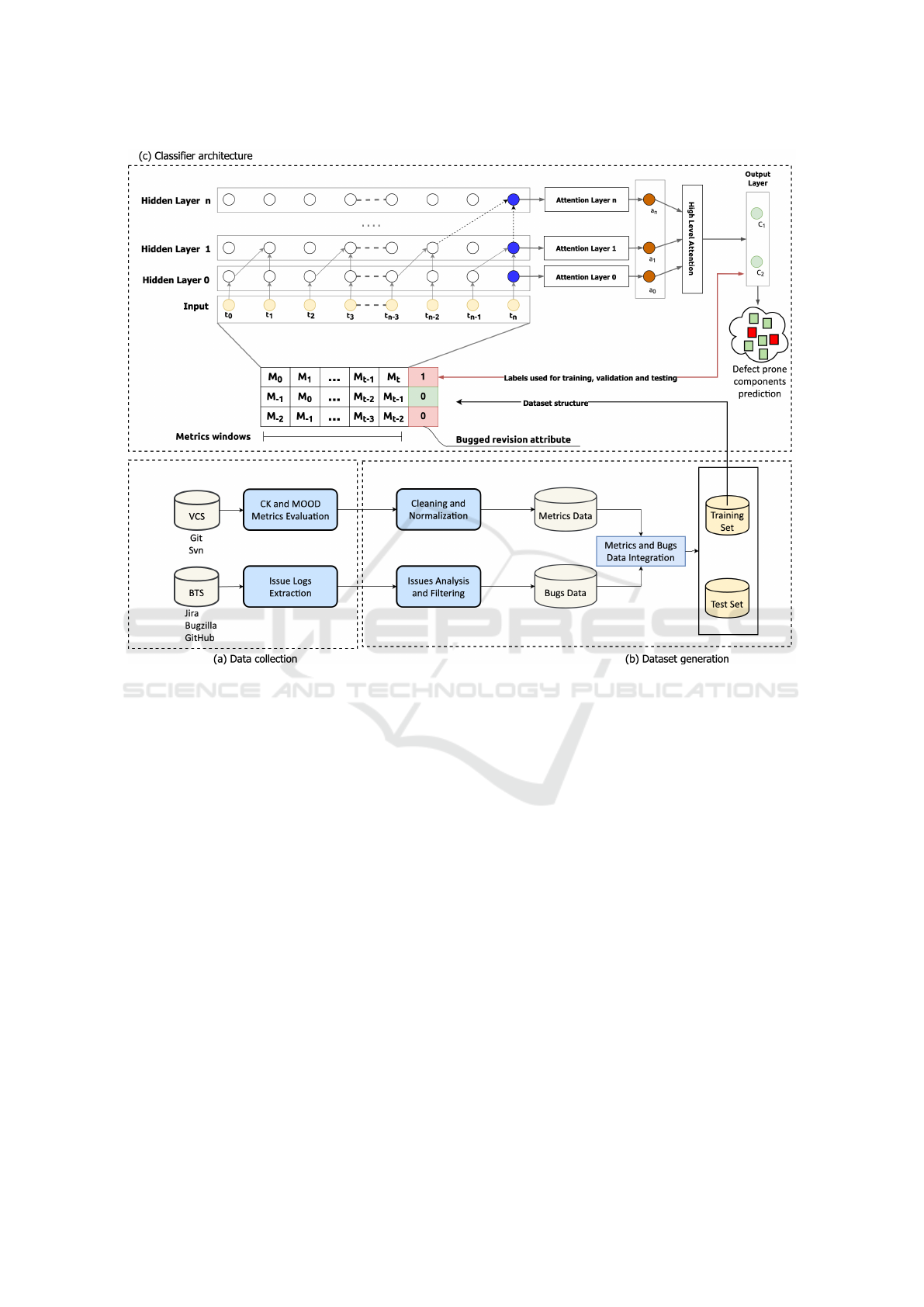
Figure 1: Overall process and classiﬁer architecture.

of issues (e.g., improvement, enhancements, feature

additions, and refactoring tasks). This is needed to

identify, for each class, only the issues that were re-

lated to bug ﬁxes, since we use them to tag faulty re-

visions of each class. Finally, we only consider issues

having the status CLOSED and the resolution DONE

since their changes must be committed in the reposi-

tory and applied to the components in the context of

a commit. This allows identifying bugged classes for

each commit in the GIT repository. At the same time,

the source code at each commit has been downloaded

and analyzed for evaluating the internal quality met-

rics of Table 1 over time. To this aim, several tools

for metrics calculation have been exploited (Hilton,

2020; Aniche, 2015; Spinellis, 2005). Finally, as de-

picted in Figure 1-(b) the metrics and the bugs data,

evaluated at each commit, are merged into a uniﬁed

training and testing dataset. During this step, the raw

data-set is also cleaned by removing incomplete and

wrong samples and normalizing the attributes (min-

max normalization). The ﬁnal dataset, for each class

of the system, contains the evolution, by commits, of

the calculated metrics integrated with bug presence

information.

4.2 The Temporal Convolution Network

Classiﬁer

The classiﬁer architecture is shown in Figure 1-(c).

The convolutional operations in the TCN architec-

ture are discussed in (Bai et al., 2018). Speciﬁcally,

the TCN network exploits a 1D FCN (fully convolu-

tional network) and padding to enforce layer length

coherence. The architecture applies causal convolu-

tions to ensure that when evaluating the output at cur-

rent time t only current and past samples are consid-

ered. The dilated convolutions specify a dilation fac-

tor f

among each pair of neighboring ﬁlters. The

factor f

grows exponentially with the layer number.

If the kernel ﬁlter size is k

, the effective history at the

lower layer is (k

− 1) ∗ d, still growing exponentially

by network depth.

For classiﬁcation, the last sequential activation of

the last layer is exploited since it summarizes the in-

formation extracted from the complete sequence in

input into a single vector. Since this representation

ICSOFT 2020 - 15th International Conference on Software Technologies

388

may be too reductive for the intricate relationships

(as those present in bugs and internal quality metrics

multivariate time-series), we added a hierarchical at-

tention mechanism across network layers inspired by

(Yang et al., 2016b). As shown in Figure 1-(c), if the

TCN has n hidden layers, L

is a matrix comprised

of the convolutional activations at each layer i (with

i = 0, 1, . . . , n) deﬁned as:

= [l

, l

, ..., l

], L

∈ R

K×T

where K is the number of ﬁlters present in each layer.

Hence layer attention weight la

∈ R

1×T

can be eval-

uated as:

= so f tmax(tanh(w

))

where w

∈ R

K×1

are trainable parameter vectors. The

combination of convolutional activations for layer i

is calculated as a

= a

) where a

∈ R

K×1

and

is an activation function (we experimented with

ReLU, Mish and Swish). At the output of the hidden-

level attention layers, the convolutional activations

A = [a

, a

, ..., a

] (with A ∈ R

K×n

) are used to

calculate the last sequence representation to perform

the ﬁnal classiﬁcation:

α = so f tmax(tanh(w

A))

y = a

(Aα

)

where w ∈ R

K×1

, α ∈ R

1×K

, y ∈ R

K×1

The considered architecture can be instantiated

with a variable number of hidden layers where each

hidden layer is the same length as the input layer.

Referring to Figure 1-(c), we exploited the follow-

ing three types of layers:

• Input Layer: it represents the entry point of the

considered neural network, and it is composed of

a node for each set of features considered at a

given time;

• Hidden Layers: they are made of artiﬁcial neu-

rons, the so-called “perceptrons”. The output of

each neuron is computed as a weighted sum of its

inputs and passed through an activation function

(i.e., mish, swish, and ReLu) or a soft-plus func-

tion.

• Attention Layers: allows modeling of relation-

ships regardless of their distance in both the input

and output sequences.

• Batch Normalization: Batch normalization is

added to improve the training of deep feed-

forward neural networks as discussed in (Ioffe and

Szegedy, 2015).

• Output Layer: this layer produces the requested

output.

The TCN training is performed by deﬁning a set of

labeled traces T = (M, l), where each of the M rows

is an instance associated with a binary label l, which

speciﬁes if a class is bugged or not as exempliﬁed in

Figure 1-(c). For each of the M instances, the process

computes a feature vector V

submitted to the classi-

ﬁer in the training phase. In order to perform valida-

tion during the training step, 10-fold cross-validation

is used (Stone, 1974). The trained classiﬁer is as-

sessed using the real data contained in the test set

made of classes (and hence bugs) that classiﬁer has

never seen.

During the training step, different parameters of

the architecture are tested (i.e., number of layers,

batch size, optimization algorithm, and activation

functions) in order to achieve the best possible per-

formance as further detailed in the next section.

The considered TCNs architecture was trained by

using cross-entropy (Mannor et al., 2005) as a loss

function, whose optimization is achieved by means of

stochastic gradient descent (SGD) technique. Speciﬁ-

cally, we adopted a momentum of 0.09 and a ﬁxed de-

cay of 1e

−6

. To improve learning performances, SGD

has been conﬁgured into all experiments with Nes-

terov accelerated gradient (NAG) correction to avoid

excessive changes in the parameter space, as speciﬁed

in (Sutskever et al., 2013).

5 EXPERIMENT DESCRIPTION

The experimentation is conducted by using the feature

model and the TCN classiﬁer described in Section 4.

Speciﬁcally, the tool-chain described in Figure 1

is applied to four different Java open-source projects.

The projects are selected by considering the neces-

sity to generalize the obtained results. However, as

discusses in (Hall et al., 2012), the data-sets, used in

the empirical investigation strongly affect prediction

performance. For this reason, the selected projects

differ for their application domain, size, number of

revisions. Table 2 describes their characteristics: the

total number of commits analyzed for each project,

the total number of bugs ﬁxed and detected for each

project, the analyzed period represented by the date

of the ﬁrst and the last commit detected.

All the projects in the table, have an available Git

repository that is active and contains more than one

release. Finally, the considered systems are also used

in other studies allowing to easily evaluate and com-

pare the obtained results.

The assessment is conducted by identifying the

best parameters reported in Table 3 found us-

ing a Sequential Bayesian Model-based Optimiza-

Temporal Convolutional Networks for Just-in-Time Software Defect Prediction

389

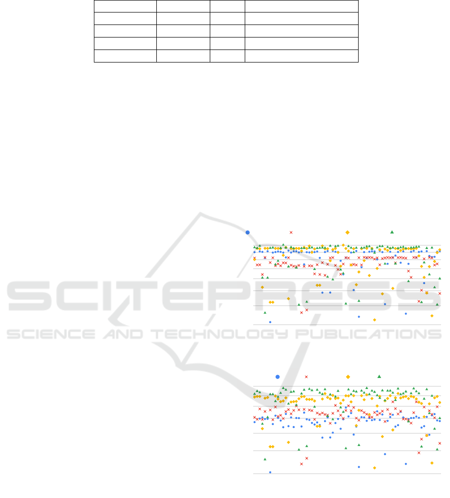
Table 2: Analysed Software Systems.

System Commits Bugs Period

Log4j 3275 647 2001-02-28/2015-06-04

Javassist 888 260 2004-07-08/2019-10-14

JUnit4 2397 153 2001-04-01/2019-04-03

ZooKeeper 1939 1787 2008-06-24/2019-10-10

tion (SBMO) approach implemented using the Tree

Parzen Estimator (TPE) algorithm as deﬁned in

(Bergstra et al., 2011).

The parameters reported in the table are the fol-

lowing:

• Network Size: we considered two levels of net-

work sizes (small, medium), depending on the ac-

tual number of layers. A small size consists of a

maximum of 1.5 mln of learning parameters. The

medium size is composed of a number of param-

eters between 1.5 mln and 7 mln;

• Activation Function: we tested three different ac-

tivations functions: Swish and Mish (Ramachan-

dran et al., 2017) in addition to the well-known

ReLu;

• Learning Rate: it ranges from 0.09 to 0.1;

• Number of Layers: the numbers of considered

layers is 6,7,9;

• Batch Size: batch size belongs to the set

{64, 128, 264} and is handled, for a multi-GPU

system, as suggested in (Koliousis et al., 2019);

• Optimization Algorithm: we tested the Stochas-

tic Gradient Descent (SGD) (Schaul et al., 2013),

RmsProp (Wang et al., 2019), Nadam (Wang

et al., 2019).

• Dropout rate: it is ﬁxed to 0.15.

The experiments run on the TensorFlow 2.1 deep

learning platform and used PyTorch 1.4 as a machine

learning library. The hardware environment of the

platform is a workstation with one dual-core micro-

processor: two Intel (R) Core (TM) i9 CPU 4.30 GHZ

64GB of RAM, one equipped with NVIDIA Tesla T4

AI Inferencing GPU and the other with Nvidia Titan

Xp.

6 DISCUSSION OF RESULTS

The plot depicted in Figure 2 shows the distribution

of (a) accuracy and (b) F-measure over the hyper-

parameters conﬁgurations. As the ﬁgure shows, the

worst results are obtained for projects having a lower

number of detected bug (e.g. Javassist and JUnit4),

while satisfactory results are obtained considering

data-set with a large number of detected bugs (e.g.,

Log4J and Zookeeper). The parameters permutations

providing the best accuracy and F-measure by the

project are listed in Table 4. Most of the models be-

have consistently and there are quite small differences

among networks with six and seven layers. It’s also

interesting to observe that there is a small set of mod-

els that are not able to learn from the data and looking

carefully at those models they fall into two categories:

(i) models with more than nine layers and medium

sizes; (ii) models trained with learning rates higher

than 0.015. For the ﬁrst case increasing the dataset is

needed and it is likely to improve ﬁnal performances.

Configurations

0.3

0.4

0.5

0.6

0.7

0.8

0.9

Accuracy-Junit Accuracy-JavaAssist Accuracy-Log4j Accuracy-Zookeeper

(a)

Configurations

0.3

0.4

0.5

0.6

0.7

0.8

0.9

F1-Junit F1-JavaAssist F1-Log4J F1-Zookeper

(b)

Figure 2: Scatter plots of distributions of accuracy (a) and

F-measure (b) for each model conﬁguration comparing ob-

tained results on the four analyzed systems.

ICSOFT 2020 - 15th International Conference on Software Technologies

390

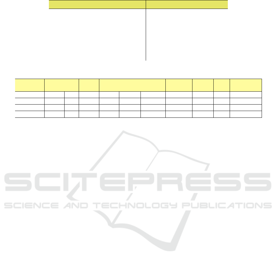
Table 3: Hyper-parameters Optimization and selected ranges.

Hyperparameters Ranges

Network size Small, Medium

Activation Function (AF) Mish, ReLu, Swish

Learning Rate (LR) [0.09, 0.12]

Number of layers { 6, 7, 8, 9 }

Batch size { 64, 128, 256 }

Optimization Algorithm (OA) SGD, Nadam, RMSprop

Table 4: Permutations providing the best validation accuracy for each project.

Project AF LR

No.

Layers

Batch

size

Dropout

Rate

Accuracy Loss F1

Training

Time (sec)

Log4j mish 9 7 64 SGD 0.15 0.996 0.0512 0.81 10275.51

Javassist mish 9 6 64 SGD 0.15 0.822 0.1770 0.72 2791.87s

JUnit4 mish 9 8 64 Nadam 0.15 0.916 0.0597 0.65 4534.22s

ZooKeeper ReLu 9 6 64 SGD 0.15 0.997 0.0002 0.87 6159.53

7 THREATS TO VALIDITY

In this section, the threats to the validity of the re-

search proposed are discussed.

Construct Validity: A threat to construct valid-

ity concerns with the source code measurements per-

formed. To mitigate this threat, we used three publicly

available tools (Hilton, 2020; Aniche, 2015; Spinellis,

2005). We decided to use more than one tool to check,

whenever possible if the measures obtained from one

tool are the same calculated by the other ones. More-

over, the fact that both the tools and the OSSs are pub-

licly available makes possible to replicate the mea-

surement task in other studies. Another threat con-

cerns with the class imbalance problem often encoun-

tered in SDP. In order to ensure that the results would

not have been biased by confounding effects of data

unbalance we adopted the SMOTE technique as de-

scribed in (Chawla et al., 2002).

Internal Validity: Threat to internal validity con-

cerns whether the results in our study correctly follow

from our data. Particularly, whether the metrics are

meaningful to our conclusions and whether the mea-

surements are adequate. To this aim, an accurate pro-

cess for the data gathering has been performed.

External Validity: Threat to external validity con-

cerns the generalization of obtained results. To mit-

igate this threat, in our investigation we considered

well-known OSS systems that are continuously evolv-

ing and different for dimensions, domain, size, time-

frame, and the number of commits. However, our re-

sults can not be generalized to commercial systems

due to the existing differences between OSS systems

and commercial systems such as the nature of re-

ported defects. In OSS systems, defects can be re-

ported by customers, for stable releases, and by de-

velopers during development activities. In commer-

cial projects, instead, the defects modeled and there-

fore studied are only those reported by customers for

released versions. Moreover, we limited our inves-

tigation to Java systems because the tools exploited

to compute the considered metrics only work for this

programming language. Thus, we cannot claim gen-

eralization concerning systems written in different

languages as well as to projects belonging to indus-

trial environments.

8 CONCLUSIONS AND FUTURE

WORK

In this work, we deﬁned a deep learning approach

based on temporal convolutional networks for just-in-

time defect prediction. To predict changes that will

introduce software defects, we used a ﬁne-grained

quality metrics features model. The approach exploits

a large data-set, from four open-source projects, with

the assessment of 33 class level source code metrics

detected commit by commit. The evaluation carried

out shows that the predictions performed with our

approach are satisfactory and the accuracy obtained

is greater than the 0.90 in most cases, achieving the

0.99 value in the case of the ZooKeeper and Log4J

projects. To our knowledge, it is the best result in re-

lated literature. However, a limit of our work is that

our model, like all prediction models, requires a large

amount of historical data to train a model that will per-

Temporal Convolutional Networks for Just-in-Time Software Defect Prediction

391

form well. In practice, training data may not be avail-

able for projects in the initial development phases, or

for legacy systems that do not have archived histor-

ical data. For this reason, in the future, we plan to

apply our approach in a cross-project context, where

models can be trained using historical data from other

projects. Moreover, we intend to extend the set of

metrics considered as features also including process

metrics. Finally, we plan to evaluate the effectiveness

of our model in-ﬁeld, through a controlled study with

practitioners to make defect prediction more action-

able in practice and support in real-time development

activities, such as code writing and code inspections.

REFERENCES

A. Ackerman, L. B. and Lewski, F. (1989). Software inspec-

tions: An effective veriﬁcation process. IEEE Soft-

ware, 6:31–36.

Aniche, M. (2015). Java code metrics calculator (CK).

Available in https://github.com/mauricioaniche/ck/.

Ardimento, P., Bernardi, M. L., and Cimitile, M. (2018). A

multi-source machine learning approach to predict de-

fect prone components. In Proceedings of the 13th In-

ternational Conference on Software Technologies, IC-

SOFT 2018, Porto, Portugal, July 26-28, 2018, pages

306–313.

Bai, S., Kolter, J. Z., and Koltun, V. (2018). An em-

pirical evaluation of generic convolutional and re-

current networks for sequence modeling. CoRR,

abs/1803.01271.

Basili, V. R., Briand, L. C., and Melo, W. L. (1996). A

validation of object-oriented design metrics as quality

indicators. IEEE Trans. Software Eng., 22(10):751–

761.

Bergstra, J., Bardenet, R., Bengio, Y., and K

egl, B. (2011).

Algorithms for hyper-parameter optimization. In Pro-

ceedings of the 24th International Conference on Neu-

ral Information Processing Systems, NIPS11, page

25462554, Red Hook, NY, USA. Curran Associates

Inc.

Bernardi, M. L., Cimitile, M., Martinelli, F., and Mercaldo,

F. (2019). Keystroke analysis for user identiﬁcation

using deep neural networks. In 2019 International

Joint Conference on Neural Networks (IJCNN), pages

1–8.

Bernardi, M. L. and Di Lucca, G. A. (2007). An interproce-

dural aspect control ﬂow graph to support the mainte-

nance of aspect oriented systems. In 2007 IEEE Inter-

national Conference on Software Maintenance, pages

435–444.

Brito e Abreu, F. and Melo, W. (1996). Evaluating the im-

pact of object-oriented design on software quality. In

Proceedings of the 3rd International Software Metrics

Symposium, pages 90–99.

Cabral, G. G., Minku, L. L., Shihab, E., and Mujahid,

S. (2019). Class imbalance evolution and veriﬁca-

tion latency in just-in-time software defect prediction.

In Proceedings of the 41st International Conference

on Software Engineering, ICSE 2019, Montreal, QC,

Canada, May 25-31, 2019, pages 666–676.

Chawla, N. V., Bowyer, K. W., Hall, L. O., and Kegelmeyer,

W. P. (2002). Smote: Synthetic minority over-

sampling technique. J. Artif. Int. Res., 16(1):321357.

Chen, X., Zhao, Y., Wang, Q., and Yuan, Z. (2018). Multi:

Multi-objective effort-aware just-in-time software de-

fect prediction. Information and Software Technology,

93:1–13.

Chidamber, S. R. and Kemerer, C. F. (1994). A metrics

suite for object oriented design. IEEE Trans. Software

Eng., 20(6):476–493.

Chidamber, S. R. and Kemerer, C. F. (1994). A metrics

suite for object oriented design. IEEE Transactions

on Software Engineering, 20(6):476–493.

Deng, L., Yu, D., et al. (2014). Deep learning: methods

and applications. Foundations and Trends

 in Signal

Processing, 7(3–4):197–387.

Fischer, M., Pinzger, M., and Gall, H. (2003). Populating a

release history database from version control and bug

tracking systems. In 19th International Conference

on Software Maintenance (ICSM 2003), The Architec-

ture of Existing Systems, 22-26 September 2003, Ams-

terdam, The Netherlands, pages 23–. IEEE Computer

Society.

Hall, T., Beecham, S., Bowes, D., Gray, D., and Counsell,

S. (2012). A systematic literature review on fault pre-

diction performance in software engineering. IEEE

Trans. Software Eng., 38(6):1276–1304.

Hassan, A. E. (2009). Predicting faults using the complexity

of code changes. In 31st International Conference on

Software Engineering, ICSE 2009, May 16-24, 2009,

Vancouver, Canada, Proceedings, pages 78–88.

Hilton, R. (2009 (accessed January 16, 2020)). Ja-

SoMe: Java Source Metrics. Available in

https://github.com/rodhilton/jasome.

Hoang, T., Dam, H. K., Kamei, Y., Lo, D., and Ubayashi,

N. (2019). Deepjit: an end-to-end deep learning

framework for just-in-time defect prediction. In 2019

IEEE/ACM 16th International Conference on Mining

Software Repositories (MSR), pages 34–45. IEEE.

Ioffe, S. and Szegedy, C. (2015). Batch normalization: Ac-

celerating deep network training by reducing internal

covariate shift. In Proceedings of the 32Nd Inter-

national Conference on International Conference on

Machine Learning - Volume 37, ICML’15, pages 448–

456. JMLR.org.

Kamei, Y., Fukushima, T., McIntosh, S., Yamashita,

K., Ubayashi, N., and Hassan, A. E. (2016).

Studying just-in-time defect prediction using cross-

project models. Empirical Software Engineering,

21(5):2072–2106.

Kamei, Y., Shihab, E., Adams, B., Hassan, A. E., Mockus,

A., Sinha, A., and Ubayashi, N. (2013). A large-

scale empirical study of just-in-time quality assur-

ance. IEEE Trans. Software Eng., 39(6):757–773.

Koliousis, A., Watcharapichat, P., Weidlich, M., Mai, L.,

Costa, P., and Pietzuch, P. (2019). Crossbow: Scal-

ICSOFT 2020 - 15th International Conference on Software Technologies

392

ing deep learning with small batch sizes on multi-gpu

servers. Proc. VLDB Endow., 12(11):13991412.

Manjula, C. and Florence, L. (2019). Deep neural net-

work based hybrid approach for software defect pre-

diction using software metrics. Cluster Computing,

22(4):9847–9863.

Mannor, S., Peleg, D., and Rubinstein, R. (2005). The cross

entropy method for classiﬁcation. In Proceedings

of the 22Nd International Conference on Machine

Learning, ICML ’05, pages 561–568, New York, NY,

USA. ACM.

Myers, G. J. and Sandler, C. (2004). The Art of Software

Testing. John Wiley & Sons, Inc., Hoboken, NJ, USA.

Pascarella, L., Palomba, F., and Bacchelli, A. (2019). Fine-

grained just-in-time defect prediction. Journal of Sys-

tems and Software, 150:22–36.

Phan, A. V., Nguyen, M. L., and Bui, L. T. (2018). Convo-

lutional neural networks over control ﬂow graphs for

software defect prediction. CoRR, abs/1802.04986.

Ramachandran, P., Zoph, B., and Le, Q. V. (2017). Search-

ing for activation functions. CoRR, abs/1710.05941.

Schaul, T., Antonoglou, I., and Silver, D. (2013). Unit tests

for stochastic optimization.

Spinellis, D. (2005). Tool writing: a forgotten art? (soft-

ware tools). IEEE Software, 22(4):9–11.

Stone, M. (1974). Cross-validatory choice and assessment

of statistical predictions. Roy. Stat. Soc., 36:111–147.

Sutskever, I., Martens, J., Dahl, G., and Hinton, G. (2013).

On the importance of initialization and momentum

in deep learning. In Proceedings of the 30th Inter-

national Conference on International Conference on

Machine Learning - Volume 28, ICML’13, pages III–

1139–III–1147. JMLR.org.

Wang, T., Zhang, Z., Jing, X., and Zhang, L. (2016). Multi-

ple kernel ensemble learning for software defect pre-

diction. Autom. Softw. Eng., 23(4):569–590.

Wang, Y., Liu, J., Mii, J., Mii, V. B., Lv, S., and Chang,

X. (2019). Assessing optimizer impact on dnn model

sensitivity to adversarial examples. IEEE Access,

7:152766–152776.

Xu, Z., Li, S., Xu, J., Liu, J., Luo, X., Zhang, Y., Zhang, T.,

Keung, J., and Tang, Y. (2019). LDFR: learning deep

feature representation for software defect prediction.

Journal of Systems and Software, 158.

Yang, X., Lo, D., Xia, X., and Sun, J. (2017). Tlel: A two-

layer ensemble learning approach for just-in-time de-

fect prediction. Information and Software Technology,

87:206–220.

Yang, X., Lo, D., Xia, X., Zhang, Y., and Sun, J. (2015).

Deep learning for just-in-time defect prediction. In

2015 IEEE International Conference on Software

Quality, Reliability and Security, QRS 2015, Vancou-

ver, BC, Canada, August 3-5, 2015, pages 17–26.

Yang, Y., Zhou, Y., Liu, J., Zhao, Y., Lu, H., Xu, L., Xu,

B., and Leung, H. (2016a). Effort-aware just-in-time

defect prediction: simple unsupervised models could

be better than supervised models. In Proceedings

of the 24th ACM SIGSOFT International Symposium

on Foundations of Software Engineering, FSE 2016,

Seattle, WA, USA, November 13-18, 2016, pages 157–

168.

Yang, Z., Yang, D., Dyer, C., He, X., Smola, A., and Hovy,

E. (2016b). Hierarchical attention networks for docu-

ment classiﬁcation. In Proceedings of the 2016 Con-

ference of the North American Chapter of the Associa-

tion for Computational Linguistics: Human Language

Technologies, pages 1480–1489, San Diego, Califor-

nia. Association for Computational Linguistics.

Young, S., Abdou, T., and Bener, A. (2018). A replica-

tion study: just-in-time defect prediction with ensem-

ble learning. In Proceedings of the 6th International

Workshop on Realizing Artiﬁcial Intelligence Syner-

gies in Software Engineering, pages 42–47.

Temporal Convolutional Networks for Just-in-Time Software Defect Prediction

393