
A New Neural Network Feature Importance Method: Application to
Mobile Robots Controllers Gain Tuning
Ashley Hill
1
, Eric Lucet
1
and Roland Lenain
2
1
CEA, LIST, Interactive Robotics Laboratory, Gif-sur-Yvette, F-91191, France
2
Universit
´
e Clermont Auvergne, Inrae, UR TSCF, Centre de Clermont-Ferrand, F-63178 Aubi
`
ere, France
Keywords:
Machine Learning, Neural Network, Robotics, Mobile Robot, Control Theory, Gain Tuning, Adaptive
Control, Explainable Artificial Intelligence.
Abstract:
This paper proposes a new approach for feature importance of neural networks and subsequently a methodol-
ogy using the novel feature importance to determine useful sensor information in high performance controllers,
using a trained neural network that predicts the quasi-optimal gain in real time. The neural network is trained
using the Covariance Matrix Adaptation Evolution Strategy (CMA-ES) algorithm, in order to lower a given
objective function. The important sensor information for robotic control are determined using the described
methodology. Then a proposed improvement to the tested control law is given, and compared with the neural
network’s gain prediction method for real time gain tuning. As a results, crucial information about the impor-
tance of a given sensory information for robotic control is determined, and shown to improve the performance
of existing controllers.
1 INTRODUCTION
In robotic control, the search for more accurate and
more adaptive controllers have been the foundation
of research in the field. Where the controller must be
able to adapt to varying known conditions or to react
with respect to observed changes in the environment.
However, it is not trivial to know a priori which as-
pects of the perception need to be included into the
control law. As such many paths have been and are
being explored for improving control law, such as
computer vision (Ha and Schmidhuber, 2018) or state
estimators and observes (Lenain et al., 2017). %
More recent papers have shown the use of neu-
ral networks for gain prediction (Hill. et al., 2019).
Where the gain changes with respect to the perception
quality, allowing the controller to adapt to information
that was underused. Indeed, due to their nature as uni-
versal function approximators (Hornik et al., 1990),
neural networks can use most of the available sensor
information; in order to predict a quasi-optimal gain
that adapts to the changes in the perception. %
However, many tasks cannot use neural networks,
for safety reasons or in some cases for performance
reasons. Indeed, they are considered black-boxes due
to their mathematical complexity and high number
of internal parameters (LeCun et al., 2015), making
them hard to analyze and predict consistent behavior.
As such, the natural question that follows, is how
to analyze trained neural controllers in order to un-
derstand their behavior, and possibly improve current
control laws. This is an important question in the
field of machine learning and artificial intelligence in
general, and currently heavily researched (Gunning,
2017). In this paper, the application of existing and
novel analysis methods are used, in order to under-
stand the how a trained gain prediction method reacts
to its input information, and how this knowledge can
be used in order to improve classic control law.
At first, a few methods for neural network analysis
will be described, including a novel analysis method.
Then, an experimental setup, where the gain predic-
tion method is described, along with a dynamic sim-
ulation of a robotic car-like bicycle model. Followed
by experiments showing how to integrate the analysis
information into improving the control law. And fi-
nally, a discussion of the results and in depth analysis
before concluding.
188
Hill, A., Lucet, E. and Lenain, R.
A New Neural Network Feature Importance Method: Application to Mobile Robots Controllers Gain Tuning.
DOI: 10.5220/0009888501880194
In Proceedings of the 17th International Conference on Informatics in Control, Automation and Robotics (ICINCO 2020), pages 188-194
ISBN: 978-989-758-442-8
Copyright
c
2020 by SCITEPRESS – Science and Technology Publications, Lda. All rights reserved

2 ANALYSIS METHOD
2.1 Preliminaries
The analysis is based on feature importance, it de-
scribes how important each input feature is in order to
obtain a good prediction.
This is usually used in the context of decision trees
(Liaw et al., 2002), where each node on the tree has
a score determining the quality of its split. Which in
some cases is the Gini impurity (Suthaharan, 2016).
The feature importance is described as the input pa-
rameters that lead to a low Gini impurity for each
node that use the input feature for its split. When
sorted, these feature importance show which inputs
where the most useful in order to obtain a good pre-
diction.
Unfortunately, decision trees struggle to outmatch
the performance of neural networks, due to neural net-
works strengths as dimensional reducers and being
universal function approximators for non-linear func-
tions (LeCun et al., 2015). This means that in most
cases neural networks must be used in order to obtain
the desired performance.
The notion of feature importance is still available
to neural networks, however they are not as clear as
for the decision trees. The most known method is the
Temporal Permutation method, described in (Molnar,
2019), and detailed in the following section.
2.2 Feature Importance using Temporal
Permutation
Neural network predicts from a vector inputs, a de-
sired output vector. By varying the inputs and ob-
serving the change in the output, a correlation can be
established between each input and amount of change
for the output. This correlation shows if a given in-
put were to change, by how much would the output
change.
If the assumption that the neural network predicts
a quasi-optimal output is given. Then the change be-
tween the original predicted output, and the predicted
output when the input was altered, should give the in-
fluence each input has on the output. And this is turn
gives describes how important each input is to pre-
dicting the quasi-optimal output.
However, the changes that are made to each in-
put must be in such a way, that the input values
must remain consistent and realistic. For this, the ap-
proach proposed in (Molnar, 2019), use a temporal
permutation method. Where for a list of input vectors
recorded over time and a given input to analyze, the
given input will be shuffled across all the input vectors
over time. This causes a given input to be randomly
permuted over time, meaning the input value will not
longer hold any meaning with respect to the other in-
puts in the input vector. This input will then be similar
to a random distribution of the same type as observed
in the initial unshuffled input vectors.
When this method is applied to each input, a dif-
ference of the output, relative to each input can be
achieved. Where the difference of the output is di-
rectly translated to the error of the output, if the as-
sumption that the neural network predicts a quasi-
optimal output is given.
2.3 Feature Importance using the
Gradient
Feed forward multilayer perceptron neural networks,
consist of a sequence of matrix multiplications, adds,
and activation functions, from the given input to the
given output (LeCun et al., 2015):
y = a(b
(n)
+ w
(n,n−1)
a(...b
(1)
+ w
(1,0)
X))
Where y is the output, X is the input, a is the activation
function, b
(n)
is the bias at the layer n, and w
(n,n−1)
is
the weight matrix between the layer n and the layer
n − 1.
From this, the gradient between the output, and
any component of the neural network can be achieved
using the chain rule. Indeed this is the exact method
that is used in backpropagation (LeCun et al., 2015)
for gradient descent in supervised learning methods
applied to neural networks.
However, backpropagation is only used to tune the
parameter of the neural network in order to minimize
an error between the predicted output and a desired
output. A different method can be used with the chain
rule to calculate the rate of change of the output value
with respect to the input vector:
∂y
∂X
=
∂y
∂a
∂a
∂z
(n)
∂z
(n)
∂s
(n−1)
. . .
∂s
(1)
∂a
∂a
∂z
(1)
∂z
(1)
∂X
∂y
∂X
= a
0
(z
(n)
)w
(n,n−1)
. . . a
0
(z
(1)
)w
(1,0)
A variant of this method was previously used in
image modification with neural networks, in order to
change an input image that maximized a cost func-
tion (Mordvintsev et al., 2015). And for determining
a Saliency map in image classifiers (Simonyan et al.,
2013).
Using this methods a jacobian matrix between
each output component and each input component,
can be obtained at each feed forward prediction of
the neural network. With this, the average and vari-
ance of the rate of change for each input with respect
A New Neural Network Feature Importance Method: Application to Mobile Robots Controllers Gain Tuning
189
to the output can be achieved over a given task. The
contribution that allow the method to return the fea-
ture importance, is the assumption that the neural net-
work predicts a quasi-optimal output. Where the rate
of change of the output is directly translated to the
error of the output. Meaning if a low rate of change
for a given input is obtained, then the input does not
contribute much to the quasi-optimal output, and as
such is not considered to be an important feature for
the prediction method.
3 EXPERIMENTAL SETUP
Before any analysis of the neural network can be
done, a training environment must first be established.
For this, a robotic car-like model in a dynamic simu-
lation is used to generate training samples. Which are
then used as input to a covariance matrix adaptation
evolution strategy (CMA-ES) method (Hansen, 2016)
in order to optimize a neural network’s weights and
biases, to minimize an objective function. This neural
network has as a goal to output in real time, the quasi-
optimal gains for the steering controller, in a similar
fashion to previous works (Hill. et al., 2019).
3.1 Robotic Model & Simulation
The robotic model is a dynamic bicycle model, which
takes into account the slide slip angle and lateral
forces applied to the rear and front axle. This model
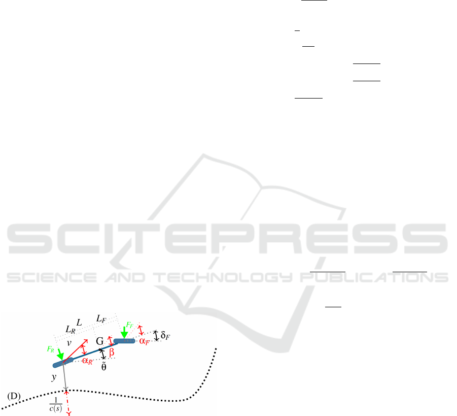
is show in the figure 1.
Figure 1: The dynamic robot model.
The notation of the model being defined as fol-
lows: (D) is the trajectory being followed, s is the
curvilinear abscissa along D, L is the wheel base
length of the robot, v is the speed vector of the robot
at the middle of the rear axle,
˜
θ is the angular error, y
is the lateral error, c(s) is the curvature at the point s,
δ
F
is the front steering angle, G is the center of mass
of the robot, L
R
and L
F
are the distance from the cen-
ter of mass to the rear and front axle respectively, F
R
and F
F
are the lateral force on the rear and front axle
respectively, β is the vehicle sliding angle, α
F
and α
R
are the front and rear axle sliding angle respectively,
I
z
is the moment of inertia across the Z axis.
From this modeling, the following system of equa-
tions can be derived:
˙s = v
cos(
˜
θ)
1−c(s)y
˙y = v sin(
˜
θ)
¨
θ =
1
I
z
(−L
F
F
F
cos(δ
F
) + L
R
F
R
)
˙
β = −
1
v
2
m
(F
F
cos(β − δ
F
) + F
R
cos(β)) −
˙
θ
β
R
= arctan(tanβ −
L
R
˙
θ
v
2
cos(β)
)
β
F
= arctan(tanβ +
L
F
˙
θ
v
2
cos(β)
) − δ
F
v
2
=
vcos(β
R
)
cos(β)
The lateral forces applied to the rear and front
axle, follow the Pacejka magic formula (Bakker et al.,
1987), in order to obtain a more realistic and dynamic
environment.
An extended Kalman filter (Welch and Bishop,
1995) is used in order to determine the robotic state
from the sensor input, along with the covariance.
The steering actuators are modeled using an action
delay of approximately 0.5s.
This robot’s steering is controlled using the fol-
lowing control equation:
δ
F
= arctan
L cos
3
ε
θ
α
k
θ
(e
θ
) +
κ
cos
2
(ε
θ
)
with e
θ
= tan ε
θ
−
k
l
ε
l
α
is the relative orientation
error of the robot to reach its trajectory (i.e. ensur-
ing the convergence of ε
l
to 0). This control detailed
in (Lenain et al., 2017) guaranties the stabilization of
the robot to its reference trajectory, providing a rele-
vant choice for the gains k
θ
and k
l
.
3.2 Gain Prediction Model & Training
The gain prediction model used, is based on previ-
ous works (Hill. et al., 2019), where a neural net-
works predicts the quasi-optimal gain that minimize
a given objective function. This neural network pre-
dict this gain using information that is underused in
the control loop, such as the perception quality. This
neural network has 3 hidden layers of 40, 100 and
10 neurons respectively, with a hyperbolic tangents
as an activation function. It is then optimized in order
to minimize the objective function using the CMA-
ES method (Hansen, 2016). The full control loop is
shown on the figure 2:
ICINCO 2020 - 17th International Conference on Informatics in Control, Automation and Robotics
190
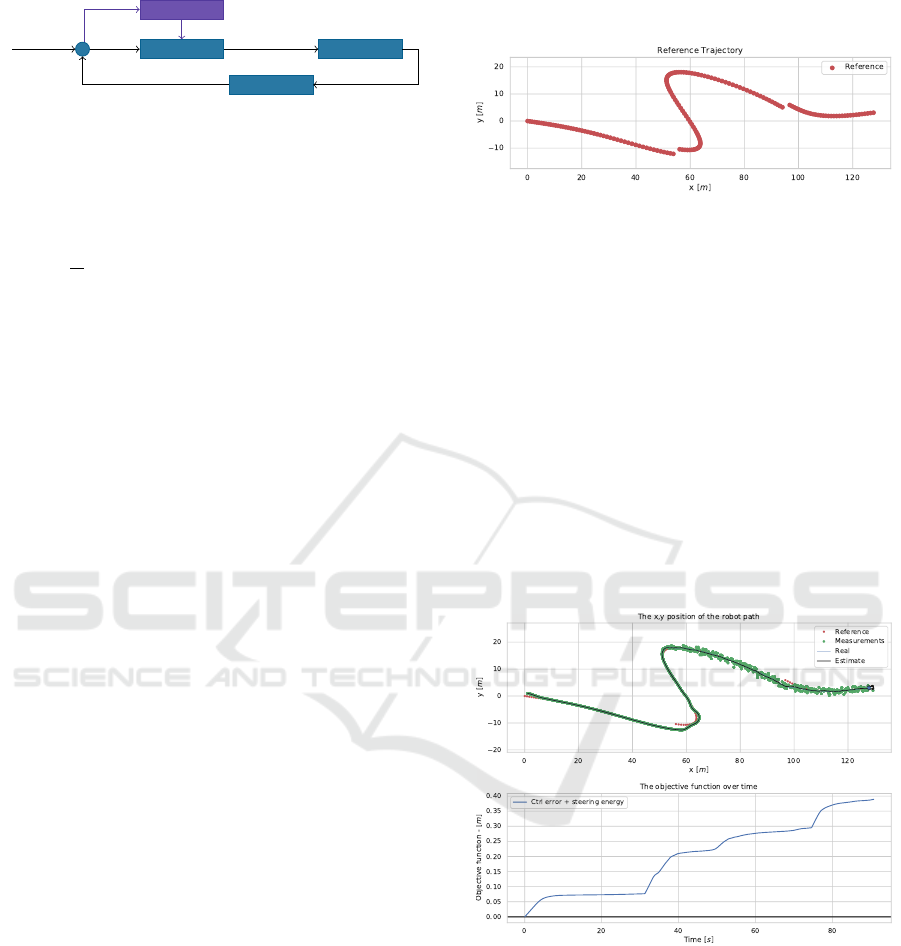
Controller
Robot
Observer
Tracking
errors
Errors
Control input
Measures
State
Gain model
Errors, state,
covariance,
curvature
Gains
Figure 2: The control loop of the mobile robot steering task,
with a gain predictor.
The objective function used is the following (de-
fined in [m]):
ob
1
=
1
T
N
∑
n=0
|y(t
n
)| + L|
˜
θ(t
n
)| + k
steer
L|δ
F
(t
n
)|
dt
Where T is the total time taken to follow the path, N is
the number of measured timesteps, t
n
is the time at the
timestep n, y is the lateral error,
˜
θ is the angular error,
δ
F
is the front steering, and dt is the time step be-
tween two samples. k
steer
is set to 0.5, as it showed to
be the ideal compromise between minimizing the con-
trol errors, and keeping a low steering energy which
minimizes oscillations.
This training was done using the previously de-
scribed simulation, over 20000 trajectory examples
using a population of 32 for CMA-ES.
3.3 Feature Importance for Robotic
Control
In robotics, there can be many sensors that can mea-
sure a wide variety of different kinds information.
However, it is not always clear what kind of infor-
mation or sensors will be of use in order to develop a
performant control equation.
As such, the goal of the following experiments, is
to use a trained neural network that can predict the
quasi-optimal gain. And from this, determine which
inputs of the neural network are used the most in order
to minimize the given objective function.
This will give a list of features that are needed in
order to improve the performance of the control equa-
tion. Some of which will then be integrated into the
control law.
4 RESULTS
The following results were obtained using the previ-
ously described methods, with a line following task
and the trajectory shown in the figure 3, at 2.0m.s
−1
,
1.5m.s
−1
, and 1.0m.s
−1
. Midway though the trajec-
tory, a GPS noise of 1m is applied to simulate a per-
ception quality loss. Two change lanes occurs along
the trajectory, in order to simulate a GPS constellation
jump or a sudden change in the target set-point.
Figure 3: The trajectory.
The method will use the trained neural network,
over the given trajectory, in order to calculate the two
feature importance methods. The temporal permu-
tation feature importance is then compared with the
novel feature importance method. Followed by an ap-
plication of the feature importance for improving the
control law.
4.1 Baseline
The baseline method that will be used to compare in
the following sections, is the expert tuned constant
gain method. Using a gain of k
l
= 0.2, and k
θ
= 1.0.
The results for the experiment can be see in the
figure 4. Where the baseline method reached an
Figure 4: Above: The method line following. Below: the
objective function over time.
end objective function value of 0.389m, 0.336m, and
0.308m for 2.0m.s
−1
, 1.5m.s
−1
, and 1.0m.s
−1
respec-
tively.
This method has some obvious shortcomings, as
it is not adaptive to the changes in speed or sensor
accuracy. Which can be observed in the noisy region,
where the controller is reacting to the GPS noise.
A New Neural Network Feature Importance Method: Application to Mobile Robots Controllers Gain Tuning
191
4.2 Gain Adaptation
The neural network gain method uses the information
in the control loop, in order to minimize the objec-
tive function. As such, it is able to predict the quasi-
optimal gain along the trajectory at any given time.
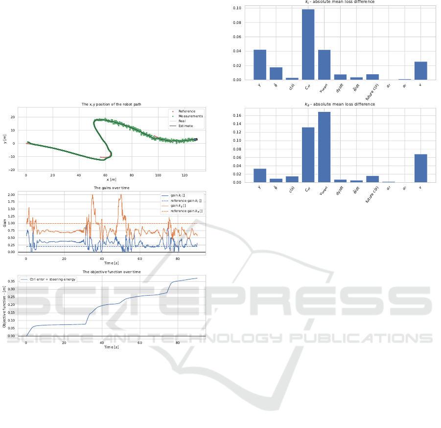
The results for the experiment can be see in the
figure 4. Where the neural network gain method
Figure 5: Above: The method line following. Middle: The
predicted gain, where the reference gain is the baseline con-
stant gain. Below: the objective function over time.
reached an end objective function value of 0.372m,
0.325m, and 0.291m for 2.0m.s
−1
, 1.5m.s
−1
, and
1.0m.s
−1
respectively.
The neural network is adapting the gain with re-
spect to changes in the speed, sensor accuracy, curva-
ture, and error. This allows the method to lower it’s
objective function substantially when compared to the
baseline method.
The feature importance can now be done over the
trained neural network. For this, both the temporal
permutation feature importance and the novel gradi-
ent feature importance are done.
On figure 6, the temporal permutation feature im-
portance can be observed. It is shown as the absolute
mean difference between the original predicted gain,
and the predicted gain when the given input is shuf-
fled over time. From this, the most important features
for both gains, from highest to lowest are the Kalman
covariance matrix denoted C
xy
, the speed and target
Figure 6: The temporal permutation feature importance.
Above: for the k
l
gain. Below: for the k
θ
gain.
speed denoted v and v
target
respectively, the lateral er-
ror denoted y, the angular error denoted
˜
θ, and the
curvature denoted c(s).
The temporal permutation feature importance de-
scribes the absolute change in the gain, with respect
to the input feature. However is it does not show the
rate of change of the gains, with respect to the val-
ues of the input features. For this the gradient feature
importance is used.
On figure 7, the gradient feature importance can
be observed. It is shown as the mean and the variance
of the jacobian matrix of the gain for each input. A
large amplitude in the jacobian for a given input, im-
plies a strong influence of the input with respect to
the output. As such, the feature importance can be
derives by ranking the input, by order of largest to
smallest amplitude.
Similarly to the temporal permutation feature im-
portance, the most important features for both gains,
from highest to lowest are the Kalman covariance ma-
trix denoted C
xy
, the speed and target speed denoted v
and v
target
respectively, the lateral error denoted y, the
angular error denoted
˜
θ, the curvature denoted c(s),
and the future curvature (the predicted curvature at
t + 1s) denoted future c(s) due to its high variance.
From this, the equivalence of the feature impor-
tance methods can be implied. However the gradient
feature importance has some strong strengths to it: It
does not need each input features to vary in order to
obtain the feature importance. Indeed if a given input
does not explore the span of values during the analy-
sis, the temporal permutation feature importance will
ICINCO 2020 - 17th International Conference on Informatics in Control, Automation and Robotics
192
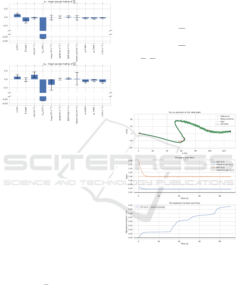
Figure 7: The gradient feature importance, as the mean ja-
cobian matrix. The figure is cut midway to avoid scaling
issue of outliers. The error bars, show the variance of the
jacobian matrix. Above: for the k
l
gain. Below: for the k
θ
gain.
not return the correct feature importance. Further-
more the gradient feature importance can return the
jacobian matrix for each input and output, at each feed
forward of the neural network. Allowing for real time
analysis and approximate prediction of the behavior
of the neural network. And finally, the mean jacobian
matrix for each input and output can be used, as an
approximation of the neural network’s behavior, that
can be exploited to improve the control equation, as
shown in the following section.
4.3 Improving Control Law
The ideal way to change the control law, is to derive
it from the model while taking some of the important
features into account (covariance, speed, sliding an-
gles, ...). However, in this case study a simple mod-
ification of the gain will be used in order to show a
proof of concept.
For this, the gains equation are augmented using
the mean jacobian
∂y
∂X
matrix for the speed. Even
though more inputs could be used to improve the con-
trol law, in this case study only the speed is exploited.
The covariance is not used for example, due to how
the neural network is using it for non-linear adapta-
tion of the gain. As such a linearization of the jaco-
bian is not a valid approximation of the original gain
behavior for the covariance, and in which during ex-
perimentation lead to unstable behavior.
Using the mean jacobian matrix, the following
gain equations are derived:
k
l
= v
∂
ˆ
k
l
∂v
+ k
lv
k
θ
= v
∂
ˆ
k
θ
∂v
+ k
θv
Where
∂
ˆ
k
l
∂v
,
∂
ˆ
k
θ
∂v
are the mean jacobian of the predicted
gains with respect to the speed, v is the longitudinal
speed, and k
lv
, k
θv
are the new tune-able gains for the
control equation. This modification should allow the
control law to change its reactivity to the error with
respect to changes in the speed.
The results for the experiment can be see in
the figure 8. Where the improved control equation
Figure 8: Above: The method line following. Middle: The
predicted gain, where the reference gain is the baseline con-
stant gain. Below: the objective function over time.
method reached an end objective function value of
0.387m, 0.327m, and 0.288m for 2.0m.s
−1
, 1.5m.s
−1
,
and 1.0m.s
−1
respectively.
The improved control is adapting the gain with re-
spect to changes in the speed. This allows the method
to lower it’s objective function substantially when
compared to the baseline method, and to achieve simi-
lar performance to the neural network gain adaptation
method. Furthermore, it is able to capture the fast ini-
tial convergence to the trajectory that the neural net-
A New Neural Network Feature Importance Method: Application to Mobile Robots Controllers Gain Tuning
193
work gain adaptation method had, thanks to the initial
speed up (visible from t = 0 to t = 5).
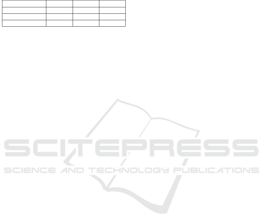
Table 1: The objective function obtained for each method
and speed over the trajectory.
1.0m.s
−1
1.5m.s
−1
2.0m.s
−1
Baseline 0.308m 0.336m 0.389m
Neural net gain 0.291m 0.325m 0.372m
Improved control 0.288m 0.327m 0.387m
In the table 1, the objective function for each
method and speed can be observed. In all cases the
baseline constant gain method had the highest ob-
jective function, meaning it had the worst perfor-
mance. For the improved control and the neural net-
work gain method, both results are comparable, as
most of the performance gained is thanks to the speed
adaption. However the improved control does not
adapt to changes in the covariance, which in some
cases allows the neural network gain method to out-
perform the improved control method.
5 CONCLUSION
A novel method for feature importance and a novel
methodology to determine useful sensor information
was proposed. This feature importance method allows
the analysis of a neural network’s behavior, to show
the importance of each sensor information, and to po-
tentially build an approximation of the neural network
for a given input.
It has been applied to a steering controller of a car-
like robot for a line following task in a highly dynamic
simulated environment. In order to analyze a gain pre-
diction method, and determine the optimal changes to
the control equations to improve its performance. In-
deed, the tested modification to the control law has
been shown to reach comparable performance to the
initial neural network gain prediction method.
This methodology can be applied to any given
simulated model of a robot control task, in order to
improve its control performance for a given criteria
encoded as a objective function.
However, the sensor information must be ide-
ally used to derive new control law from the robotic
model, as using a linear approximation for a neural
network will not encode the complete characteristic
behavior to the neural network. As such this method-
ology far more powerful as a tool to describe what is
important for control law, not how to derive a novel
control law.
Future works include validating this methodology
on varying control tasks in different field, and to use
the novel feature importance method to assist in de-
mystifying neural networks.
REFERENCES
Bakker, E., Nyborg, L., and Pacejka, H. B. (1987). Tyre
modelling for use in vehicle dynamics studies. Tech-
nical report, SAE Technical Paper.
Gunning, D. (2017). Explainable artificial intelligence
(xai). Defense Advanced Research Projects Agency
(DARPA), nd Web, 2.
Ha, D. and Schmidhuber, J. (2018). World models. arXiv
preprint arXiv:1803.10122.
Hansen, N. (2016). The CMA evolution strategy: A tutorial.
CoRR, abs/1604.00772.
Hill., A., Lucet., E., and Lenain., R. (2019). Neuroevolu-
tion with cma-es for real-time gain tuning of a car-like
robot controller. In Proceedings of the 16th Interna-
tional Conference on Informatics in Control, Automa-
tion and Robotics - Volume 1: ICINCO,, pages 311–
319. INSTICC, SciTePress.
Hornik, K., Stinchcombe, M., and White, H. (1990). Uni-
versal approximation of an unknown mapping and
its derivatives using multilayer feedforward networks.
Neural Networks, 3(5):551 – 560.
LeCun, Y., Bengio, Y., and Hinton, G. (2015). Deep learn-
ing. nature, 521(7553):436–444.
Lenain, R., Deremetz, M., Braconnier, J.-B., Thuilot, B.,
and Rousseau, V. (2017). Robust sideslip angles ob-
server for accurate off-road path tracking control. Ad-
vanced Robotics, 31(9):453–467.
Liaw, A., Wiener, M., et al. (2002). Classification and re-
gression by randomforest. R news, 2(3):18–22.
Molnar, C. (2019). Interpretable machine learning. Lulu.
com.
Mordvintsev, A., Olah, C., and Tyka, M. (2015).
Deepdream-a code example for visualizing neural net-
works. Google Research, 2(5).
Simonyan, K., Vedaldi, A., and Zisserman, A. (2013).
Deep inside convolutional networks: Visualising im-
age classification models and saliency maps.
Suthaharan, S. (2016). Decision tree learning. In Machine
Learning Models and Algorithms for Big Data Clas-
sification, pages 237–269. Springer.
Welch, G. and Bishop, G. (1995). An introduction to the
kalman filter. Technical report, Chapel Hill, NC, USA.
ICINCO 2020 - 17th International Conference on Informatics in Control, Automation and Robotics
194
