Analyzing Decision Polygons of DNN-based Classification Methods
Jongyoung Kim, Seongyoun Woo, Wonjun Lee, Donghwan Kim and Chulhee Lee
Department of Electrical and Electronic Engineering, Yonsei University,
134 Shinchon-Dong, Seodaemun-Gu, Seoul, Republic of Korea
Keywords: Decision Polygon, ReLU, Convolutional Neural Networks, Decision Boundary.
Abstract: Deep neural networks have shown impressive performance in various applications, including many pattern
recognition problems. However, their working mechanisms have not been fully understood and adversarial
examples indicate some fundamental problems with DNN-based classification methods. In this paper, we
investigate the decision modeling mechanism of deep neural networks, which use the ReLU function. We
derive some equations that show how each layer of deep neural networks expands the input dimension into
higher dimensional spaces and generates numerous decision polygons. In this paper, we investigate the
decision polygon formulations and present some examples that show interesting properties of DNN based
classification methods.
1 INTRODUCTION
Deep neural networks (DNN) have been successfully
applied in various computer vision and pattern
recognition problems, which include speech
recognition (Sainath, 2015, Amodei, 2016), object
recognition (Ouyang, 2015, Wonja, 2017, Girshick,
2014), image processing (Jin, 2017), medical imaging
(Gibson, 2018), and super-resolution. Although the
DNN-based methods have substantially
outperformed conventional methods in many fields,
the understanding of their working models is rather
limited (Radford, 2015, Yang, 2017, Zeiler, 2014,
Yosinski, 2014, 2015, Koushik, 2016, Szegedy, 2013,
Mallat, 2016).
In (Zeiler, 2014), a visualization method was
proposed, which can provide some insight into the
intermediate feature spaces and classification
operation. Also, it is observed that the first-layer
features may not be specific to a particular task, but
can be transferable to other tasks (Yosinski, 2014). In
(Yosinski, 2015), some visualization tools were
proposed, which may provide some insight and
understanding of DCN working mechanisms. In
(Koushik, 2016), the author presented some analyses
of DCN operations in the form of a framework.
The paper is organized as follows: In Section 2 we
explain how filter banks project the space into a
higher dimension space and the ReLU function
creates a higher dimensional structure. Section 3
describes the decision polygon generation when the
ReLU function is used along with some properties of
the decision polygons. Section 4 investigates
adversarial images based on the decision polygons
and subspaces. Conclusions are drawn in Section 5.
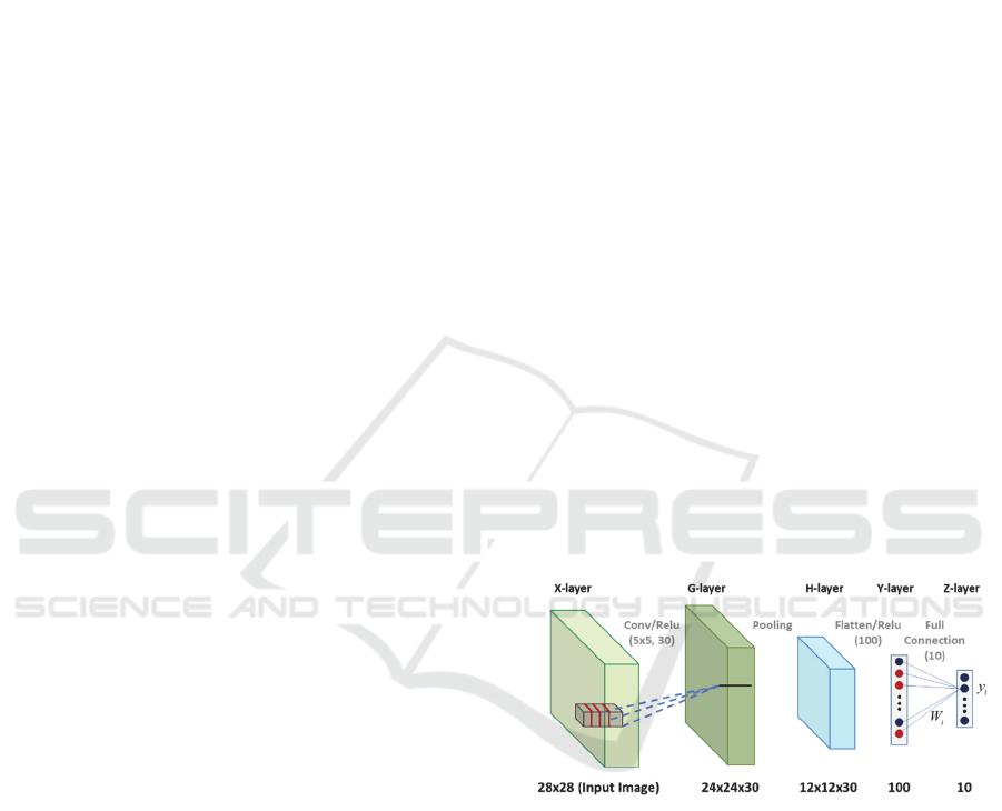
Figure 1: DCN-based classification method for the MNIST
data (softmax operation is not shown).
2 SPACE DIVISION BY FILTER
BANK
Fig. 1 shows a convolutional neural networks for the
MNIST dataset. First, thirty 2-dimensional FIR filters
(filter banks) are applied to the input hidden layers.
In this case, the FIR filters are square (e.g., 5x5). The
number of filters exceeds the number of pixels of the
window, though it can be the same as or smaller than
the number of pixels of the window. The ReLU
function is defined as follows:
346
Kim, J., Woo, S., Lee, W., Kim, D. and Lee, C.
Analyzing Decision Polygons of DNN-based Classification Methods.
DOI: 10.5220/0009888203460351
In Proceedings of the 17th International Conference on Informatics in Control, Automation and Robotics (ICINCO 2020), pages 346-351
ISBN: 978-989-758-442-8
Copyright
c
2020 by SCITEPRESS – Science and Technology Publications, Lda. All rights reserved
𝑓
𝑥
𝑚𝑎𝑥
0,𝑥
.
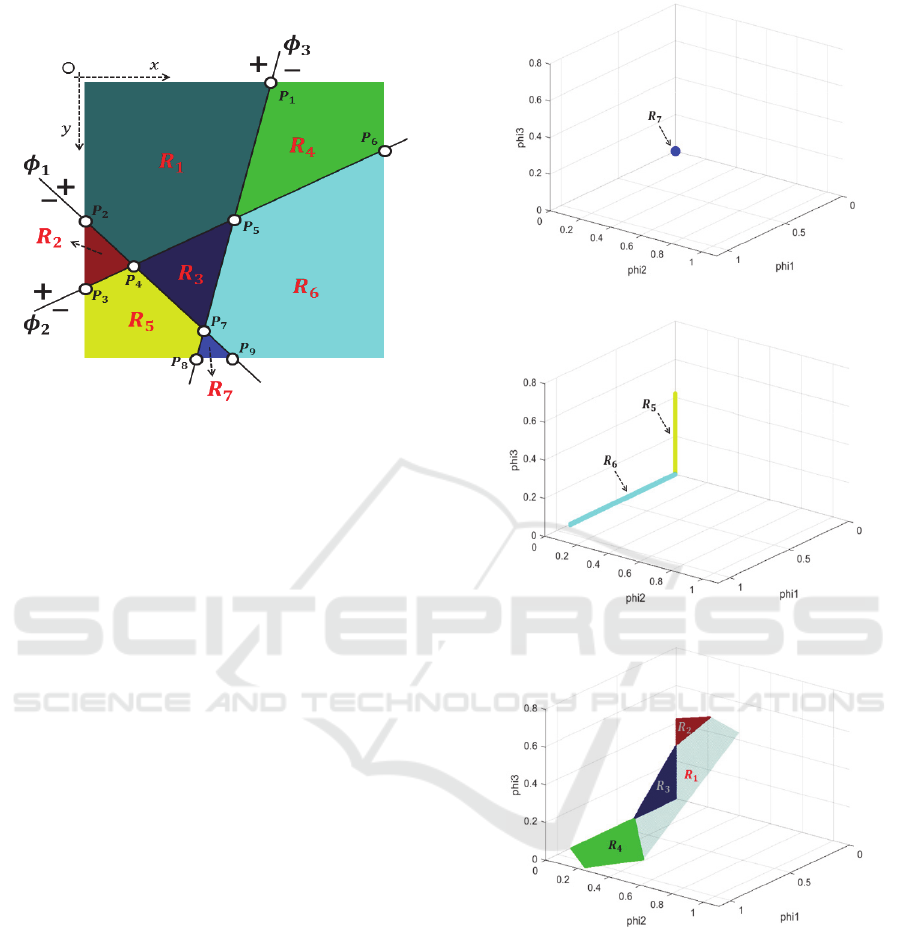
Figure 2: Three filters in the 2 dimensional space.
Fig. 2 illustrates how multiple filters with the
ReLU function perform non-linear mapping. In Fig.
2, there are three filters in the 2 dimensional input
space, which map the input space into a higher space
(3 dimensional space). The three filters can be
expressed as follows:
𝑋•𝜙
𝑐
0
𝑋•𝜙
𝑐
0
𝑋•𝜙
𝑐
0
where 𝜙
,𝜙
,𝜙
and 𝑋 are two-dimensional vectors.
In general, the three equations represent planes or
hyper-planes in high dimensional spaces and
𝜙
,𝜙
,𝜙
are the normal vectors to the planes.
The three filters divide the input space into seven
regions (Fig. 2). One region (R7) is mapped to a point
in the 3-dimensional space (Fig. 3a). Two regions
(R5, R6) are mapped into lines in the 3-dimensional
space (Fig. 3b). Three regions (R2, R3, R4) are
mapped into 2-dimensional polygons (Fig. 3c).
In region R7, we have the following relationships:
𝑋•𝜙
𝑐
0,𝑋•𝜙
𝑐
0,𝑋•𝜙
𝑐
0.
In region R5,
𝑋•𝜙
𝑐
0,𝑋•𝜙
𝑐
0,𝑋•𝜙
𝑐
0.
In region R1, we have the following:
𝑋•𝜙
𝑐
0,𝑋•𝜙
𝑐
0,𝑋•𝜙
𝑐
0.
(a)
(b)
(c)
Figure 3: Non-linear mapping of the ReLU function. (a)
Region 7 is mapped into a point, (b) Regions 5 and 6 are
mapped into lines, (c) three regions (R2, R3, R4) are
mapped into 2-dimensional polygons.
For the other regions, we can derive similar
relationships. It can be seen that a polygon in the
original input space can be mapped into a polygon in
the same dimensional space or a lower dimensional
space. Also, a polygon may have a lower degree of
freedom in the expanded space. For example, a
triangle can be mapped into a point, a line or a triangle
in the expanded space when ReLU is used in
Analyzing Decision Polygons of DNN-based Classification Methods
347
convolutional neural networks. It is also noted that a
polygon in the original space never increase its
dimension. For example, a triangle in the original
space cannot be mapped into a pyramid or a higher
dimensional polygon. At most, they can retain their
original dimension in a higher dimensional space.
However, as we can construct a three dimensional
object by folding a paper, the non-linear function of
CNN allows the original space mapped into a higher
dimensional object through the non-linear function.
Nevertheless, the local dimension in the higher space
is always the same as in the original space. For
example, although a folded paper can make a 3D
structure, locally it is always a 2D structure (plane).
3 DECISION POLYGONS OF DNN
WITH RELU
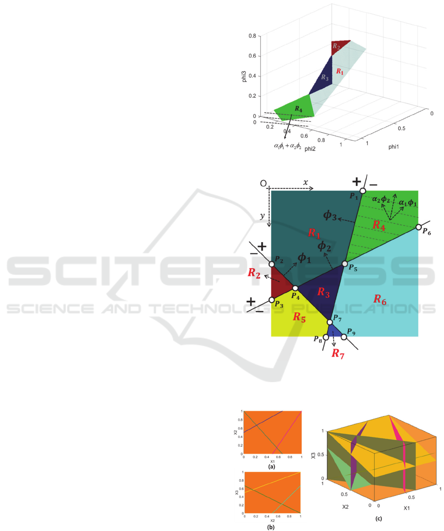
In deep convolutional networks, another filter bank or
full connection layer can be applied to the output
images. These operations can be viewed as a projection
on a vector and all the points on a plane that is normal
to the vector will be mapped into a single value (Fig.
4a). For example, if we move on the dotted line in the
expanded space (Fig. 4a), the projection value on the
vector will remain the same. Consequently, the
decision boundary will be locally linear and the
corresponding decision boundary in the original space
will be also locally linear (Fig. 4b). For example, the
decision boundary in region R4 is locally linear (a line
normal to 𝛼
𝜙
𝛼
𝜙
) and the corresponding
decision boundary in region R4 of the original input
space is locally linear (a line normal to 𝛼
𝜙
𝛼
𝜙
).
The max-pooling operation can be also viewed as
dividing a space into several subspaces. For example,
in 2 by 2 max-pooling, the maximum of four values is
selected. Consider the G-layer in Fig. 1. Without loss
of generality, we may skip the ReLU operation since
the operation doesn’t change the output of the max-
pooling operation. Thus, the max-pooling operation
chooses the maximum value among the four values
(𝐺
•𝑋
, 𝐺
•𝑋
, 𝐺
•𝑋
, 𝐺
•𝑋
):
𝐶ℎ𝑜𝑜𝑠𝑒 𝐺
•𝑋
𝑖𝑓 𝐺
•𝑋
𝐺
•𝑋
𝑖,𝑗0,..,3;𝑖𝑗.
The four vectors (𝐺
,𝐺
,𝐺
,𝐺
) represent hyper-
planes in the input space and the inequality equations
divide the input space into a number of polygons.
Therefore, the max-pooling operation will divide the
input space into a number of subspaces and all the
points of a subspace will have the same output for the
max-pooling operation. In other words, for each point
( 𝑋
) of a subspace, 𝐺
•𝑋
will be the
maximum.
(a)
(b)
Figure 4: Decision boundary formation in the expanded
space (a) and in the original space (b).
Figure 5: Space division into polygons. (a) three lines
divide the 𝑥
𝑥
space into 6 regions, (b) the same three
lines divide the 𝑥
𝑥
space into 6 regions, (c)
corresponding 3D volume divisions (polygons).
ICINCO 2020 - 17th International Conference on Informatics in Control, Automation and Robotics
348
Eventually, the original space will be divided into
a number of decision polygons and all the points
within the same polygon will be classified as the same
class when DNN with ReLU is used as a classifier
(Fig. 5). It is noted that the input dimension is very
large in typical problems and the planes defined by
the filter banks of the first layer are parallel to most
of the axes since the filter banks are highly localized.
The number of decision polygons may exceed the
number of training samples. In the MNIST dataset,
the number of training samples is 60,000 and the
number of test samples is 10,000. Table I shows the
number of samples of decision polygons. After
training the DCN of Fig. 1 using the 60,000 training
samples, we investigated the decision polygons
occupied by the training and test samples. It is found
that 69,924 decision polygons are occupied by a
single sample. Only 34 decision polygons contain
more than one sample. Also, many decision polygons
may be unoccupied.
Table 1: Number of samples within decision polygons.
No. samples per polygon No. polygons
1 69924
2 29
3 3
4 1
5 1
Recently, a number of DCN-based super
resolution methods have been proposed (Kim, 2016,
Lim, 2017, Zhang, 2018, Wang, 2018), which showed
noticeably improved performance compared to
conventional super-resolution techniques. When
DCN-based super resolution methods use the ReLU
function, the filter banks and full-connection layers
also divide the input space (receptive field) into a
large number of polygons. In this case, each image
patch can be considered as a point in the input space
and it will belong to one of the polygons. We
investigated over 22,000 image patches and found
that every image patch belonged to a different
polygon. In other words, it is observed that the
polygons generated by a DCN-based super resolution
method with ReLU are occupied by at most one
sample.
4 DECISION BOUNDARY
MARGIN OF DNN WITH RELU
4.1 Adversarial Images
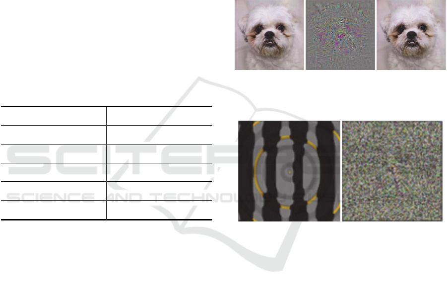
Recently, a strange behavior of DNN-based classifier
has been reported (Szegedy, 2013). A slightly
modified image may be misclassified (Fig. 6) and
such adversarial images can be easily generated to
fool DNN-based classifiers. Also, one can easily fool
DNN-based classifiers to misclassify meaningless
images with certainty (Fig. 7).
(a) (b) (c)
Figure 6: (a) original image, (b) difference image, (c)
modified image.
(a) (b)
Figure 7: (a) classified as king penguin, (b) classified as
cheetah.
4.2 Mathematical Analyses on
DNN-based Classifiers
In general, the layer dimensions are significantly
larger than the input dimension. In Fig. 1, the input
dimension is 784 (28 x 28), the G-layer dimension is
17280, the H-layer dimension is 4320 and the Y-layer
dimension is 100, the Z-layer (output layer)
dimension is 10:
𝑋𝑥
,𝑥
,...,𝑥
, 𝐺𝑔
,...,𝑔
,
𝐻ℎ
,...,ℎ
, 𝑌𝑦
,...,𝑦
,
𝑍𝑧
,...,𝑧
.
In other words, an input image is viewed as a point in
the 784 dimensional space. We can compute the
Analyzing Decision Polygons of DNN-based Classification Methods
349
gradients of each layer. The Z-layer gradients with
respect to the X-layer and the Y-layer are given by
𝛻
𝑧
≡
𝜕𝑧
𝜕𝑋
𝜕𝑧
𝜕𝑥
,…,
𝜕𝑧
𝜕𝑥
,
𝛻
𝑧
≡
𝜕𝑧
𝜕𝑌
𝜕𝑧
𝜕𝑦
,…,
𝜕𝑧
𝜕𝑦
,
𝑖 1~10
.
Although the Y-layer dimension is 100, the number
of linearly independent vectors that can affect the
outputs (𝑧
) is 10, which is equal to the number of
classes. The remaining 90 vectors that are normal to
the 10 vectors don’t affect the output values (𝑧
). We
define the subspace spanned by the 10 vectors (𝜑
)
as a relevant subspace (𝑆
) and the subspace
spanned by the 90 vectors as an irrelevant subspace
(𝑆
):
𝑆
𝑠𝑝𝑎𝑛𝜑
𝑆
𝑠𝑝𝑎𝑛𝜓
(
𝜑
•𝜓
0).
where i and j are vector indexes, and k is the layer
index.
In each layer, the layer space can be divided
into relevant and irrelevant subspaces and the
dimension of relevant space can’t exceed the number
of classes. When a sample moves in irrelevant
subspaces, all the output values (𝑧
, i = 0,..,9) remain
the same. Consequently, one can almost unlimitedly
generate equivalent images, many of which can be
meaningless images.
In the previous section, it is shown that DNN-
based classifiers divide the input space into a large
number of decision polygons and each decision
polygon is very sparsely populated. In other words,
most polygons may be unoccupied by training or test
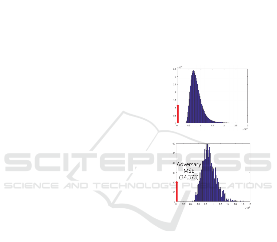
samples It is observed that the margin between a
sample and the boundaries of decision polygons is
very small (Woo, 2018). Fig. 8 shows the within-class
MSE histogram and the between-class MSE
histogram, which indicate the margins between
samples and the boundaries of decision polygons.
5 CONCLUSIONS
In this paper, we investigate the working mechanism
of DNN-based classifiers. When filter bank or full-
connection layers are applied along with the ReLU
function to a layer, the layer space is divided into a
number of polygons. Eventually, the input space is
divided into a large number of decision polygons.
Several interesting properties are observed. A vast
majority of decision polygons are occupied by a
single sample and the margin between the sample and
the boundaries of the decision polygon is very small.
In the layer space, the dimension of the relevant
subspace exceeds the dimension of the irrelevant
subspace in most cases. Consequently, in current
structures of DNN-based classifiers, it is difficult to
prevent misclassification of adversarial images. In
particular, to effectively handle adversarial images,
new type of DNN-based methods may be needed,
which provide larger margins between samples and
the boundaries of decision polygons and adequate
controls of irrelevant subspaces.
(a)
(b)
Figure 8: (a) within-class MSE histogram, (b) between–
class MSE histogram.
ACKNOWLEDGEMENTS
This research was supported by Basic Science
Research Program through the National Research
Foundation of Korea (NRF) funded by the Ministry
of Education, Science and Technology
(2017R1D1A1B03036172).
REFERENCES
Sainath, T. N., Kingsbury, B., Saon, G., Soltau, H.,
Mohamed, A. R., Dahl, G., & Ramabhadran, B. (2015).
Deep convolutional neural networks for large-scale
speech tasks. Neural Networks, 64, 39-48.
ICINCO 2020 - 17th International Conference on Informatics in Control, Automation and Robotics
350

Ouyang, W., Wang, X., Zeng, X., Qiu, S., Luo, P., Tian, Y.,
& Tang, X. (2015). Deepid-net: Deformable deep
convolutional neural networks for object detection. In
Proceedings of the IEEE conference on computer vision
and pattern recognition (pp. 2403-2412).
Jin, K. H., McCann, M. T., Froustey, E., & Unser, M.
(2017). Deep convolutional neural network for inverse
problems in imaging. IEEE Transactions on Image
Processing, 26(9), 4509-4522.
Woo, S., & Lee, C. L. (2018, August). Decision boundary
formation of deep convolution networks with relu. In
2018 IEEE 16th Intl Conf on Dependable, Autonomic
and Secure Computing, 16th Intl Conf on Pervasive
Intelligence and Computing, 4th Intl Conf on Big Data
Intelligence and Computing and Cyber Science and
Technology Congress
(DASC/PiCom/DataCom/CyberSciTech) (pp. 885-
888). IEEE.
Wojna, Z., Gorban, A. N., Lee, D. S., Murphy, K., Yu, Q.,
Li, Y., & Ibarz, J. (2017, November). Attention-based
extraction of structured information from street view
imagery. In 2017 14th IAPR International Conference
on Document Analysis and Recognition (ICDAR) (Vol.
1, pp. 844-850). IEEE.
Gibson, E., Li, W., Sudre, C., Fidon, L., Shakir, D. I.,
Wang, G., ... & Whyntie, T. (2018). NiftyNet: a deep-
learning platform for medical imaging. Computer
methods and programs in biomedicine, 158, 113-122.
Amodei, D., Ananthanarayanan, S., Anubhai, R., Bai, J.,
Battenberg, E., Case, C., ... & Chen, J. (2016, June).
Deep speech 2: End-to-end speech recognition in
english and mandarin. In International conference on
machine learning (pp. 173-182).
Girshick, R., Donahue, J., Darrell, T., & Malik, J. (2014).
Rich feature hierarchies for accurate object detection
and semantic segmentation. In Proceedings of the IEEE
conference on computer vision and pattern recognition
(pp. 580-587).
Radford, A., Metz, L., & Chintala, S. (2015). Unsupervised
representation learning with deep convolutional
generative adversarial networks. arXiv preprint
arXiv:1511.06434.
Yang, H. F., Lin, K., & Chen, C. S. (2017). Supervised
learning of semantics-preserving hash via deep
convolutional neural networks. IEEE transactions on
pattern analysis and machine intelligence, 40(2), 437-
451.
Zeiler, M. D., & Fergus, R. (2014, September). Visualizing
and understanding convolutional networks. In
European conference on computer vision (pp. 818-
833). Springer, Cham.
Yosinski, J., Clune, J., Bengio, Y., & Lipson, H. (2014).
How transferable are features in deep neural networks?.
In Advances in neural information processing systems
(pp. 3320-3328).
Yosinski, J., Clune, J., Nguyen, A., Fuchs, T., & Lipson, H.
(2015). Understanding neural networks through deep
visualization. arXiv preprint arXiv:1506.06579.
Koushik, J. (2016). Understanding convolutional neural
networks. arXiv preprint arXiv:1605.09081.
Szegedy, C., Zaremba, W., Sutskever, I., Bruna, J., Erhan,
D., Goodfellow, I., & Fergus, R. (2013). Intriguing
properties of neural networks. arXiv preprint
arXiv:1312.6199.
Mallat, S. (2016). Understanding deep convolutional
networks. Philosophical Transactions of the Royal
Society A: Mathematical, Physical and Engineering
Sciences, 374(2065), 20150203.
Kim, J., Kwon Lee, J., & Mu Lee, K. (2016). Accurate
image super-resolution using very deep convolutional
networks. In Proceedings of the IEEE conference on
computer vision and pattern recognition (pp. 1646-
1654).
Lim, B., Son, S., Kim, H., Nah, S., & Mu Lee, K. (2017).
Enhanced deep residual networks for single image
super-resolution. In Proceedings of the IEEE
conference on computer vision and pattern recognition
workshops (pp. 136-144).
Zhang, Y., Li, K., Li, K., Wang, L., Zhong, B., & Fu, Y.
(2018). Image super-resolution using very deep residual
channel attention networks. In Proceedings of the
European Conference on Computer Vision (ECCV) (pp.
286-301).
Wang, X., Yu, K., Wu, S., Gu, J., Liu, Y., Dong, C., ... &
Change Loy, C. (2018). Esrgan: Enhanced super-
resolution generative adversarial networks. In
Proceedings of the European Conference on Computer
Vision (ECCV) (pp. 0-0).
Analyzing Decision Polygons of DNN-based Classification Methods
351
