
Towards Fully Automated Inspection of Large Components with UAVs:
Offline Path Planning
Constantin Wanninger
a
, Raphael Katschinsky, Alwin Hoffmann
b
, Martin Sch
¨
orner
c
and Wolfgang Reif
Institute for Software and Systems Engineering, University of Augsburg, Augsburg, Germany
Keywords:
UAV, Visual Inspection, Trajectory Planning, Ant Colony Optimization.
Abstract:
Automation mechanisms are increasingly established in the field of visual inspections. UAVs can be used
for particularly large components, such as those used in ship production and for critical infrastructures. This
paper concentrates on the problem of visual inspection in the field of perspective-dependent route planning.
It is shown how the requirements for such a system can be implemented and elaborated. Furthermore we
investigate how sensor positions can be calculated offline, based on optical and geometrical requirements
and how a trajectory can be planned which contains the found sensor positions for each given area on the
component. It is shown how the systems architecture can be designed in order to be able to adapt it to
different requirements for the planning of sensor positions and trajectory. The implementation was tested in
a simulation environment, evaluated using a benchmark data set and it was shown how above-average results
can be achieved on this data set.
1 INTRODUCTION
The development progress and the strongly increased
availability of unmanned aerial vehicles (UAVs) in
the last years open up more and more possibilities
for civil and scientific applications. For example, the
use of UAVs for the inspection and measurement of
infrastructures is being investigated, as they enable
image-based observation from almost any perspec-
tive. Among others, the Competence Center Multi-
copter of (Deutsche Bahn AG, 2020) offers a com-
prehensive portfolio in the infrastructure sector. This
includes the inspection of rail tracks, buildings and
bridges as well as construction progress and condition
documentation, to name just a few.
A still little explored area, is the fully automated
visual inspection of large technical components by
UAVs, to which this work is dedicated. The com-
ponents considered here are assemblies according to
DIN-199, i.e. self-contained objects consisting of at
least two individual parts or assemblies of lower or-
der. Currently, visual inspection of large technical
components is still mostly carried out manually. For
a
https://orcid.org/0000-0001-8982-4740
b
https://orcid.org/0000-0002-5123-3918
c
https://orcid.org/0000-0001-6237-222X
this purpose, an inspector checks the attached individ-
ual parts whether the present situation corresponds to
the normal conditions of the component. This form of
inspection, however, is associated with longer inspec-
tion times, increased personnel expenditure, human
error susceptibility, and thus with overall increased fi-
nancial costs, which can be addressed by the full au-
tomation of the visual inspection.
The offline path planning within a fully automated
inspection is usually divided into two subproblems,
finding sensor positions, so-called viewpoints, and
finding a collision-free route through all viewpoints.
When planning viewpoints, it must be ensured that
they can be reached by the UAV and that no obsta-
cles block the view of the component to be examined,
or more generically expressed point of interest (POI).
In order for a POI, e.g, to be optimally located in the
picture, the desired resolution, focus and the camera’s
angle of aperture must be taken into account when
choosing the location of the viewpoint in relation to
the POI. When selecting the position, the orientation
of the visual sensor to the normal of the POI must
also be taken into account. However, this desired ori-
entation cannot necessarily be achieved with a UAV,
since the tilt and inclination angle of the UAV can-
not be selected at will and the camera is statically
attached to the copter or the degree of freedom of a
Wanninger, C., Katschinsky, R., Hoffmann, A., Schörner, M. and Reif, W.
Towards Fully Automated Inspection of Large Components with UAVs: Offline Path Planning.
DOI: 10.5220/0009887900710080
In Proceedings of the 17th International Conference on Informatics in Control, Automation and Robotics (ICINCO 2020), pages 71-80
ISBN: 978-989-758-442-8
Copyright
c
2020 by SCITEPRESS – Science and Technology Publications, Lda. All rights reserved
71

swivel-mounted camera is limited. Therefore, it must
be considered to what extent the angle between the
normal of the POI and the vector of the optical axis
of the camera may deviate. In addition, a minimum
distance between the copter and the component may
be required for safety reasons.
The route should contain all viewpoints from
which all POIs can be inspected. Therefore, it is im-
portant to keep the route through all the viewpoints as
short as possible and optimize the route lenght. Since
the search for the shortest route in three-dimensional
space is NP-hard (LaValle, 2006), procedures must be
considered that offer an almost optimal solution for
this problem in polynomial time. In the course of op-
timizing the route length, it is therefore important to
keep the number of viewpoints as small as possible,
while still ensuring an optimal view of all POIs.
This work is dedicated to exactly these two parts,
the viewpoint and trajectory planning. This involves
the fully automated inspection of predefined areas on
the component. It is examined how viewpoints can be
planned offline on the prerequisites mentioned above
and a route based on them. The designed procedure
is tested simulatively and the results of the trajectory
planning are evaluated using benchmark data sets.
2 RELATED WORK
Work that is specifically dedicated to the fully auto-
mated inspection of technical infrastructures by UAVs
usually aims to achieve complete visual coverage
of the entire surface of the respective infrastructure,
which is the aim of the Coverage Path Planning (Gal-
ceran and Carreras, 2013; Danner and Kavraki, 2000).
A detailed summary of the current inspection scenar-
ios provided by UAVs is provided by (Jordan et al.,
2018). According to the work of (Bircher et al.,
2015), the most adaptable approaches to the inspec-
tion scenario are those that use two-step optimiza-
tion. In a first step, viewpoints are computed that
cover the entire surface of the infrastructure, which
can be achieved by solving the Art Gallery problem
(O’Rourke, 1987; Gonz
´
alez-Banos, 2001). In a sec-
ond step, a route or trajectory is calculated that con-
nects all viewpoints, which can be modeled by solv-
ing the Traveling Salesman Problem (Laporte, 1992).
A concrete CPP solution for UAVs is described
by (Bircher et al., 2015), in which the surface of
the infrastructure is represented by a triangle mesh
and a viewpoint is calculated for each triangle, from
which the triangle is completely visible. In the sec-
ond step a route through all viewpoints is planned.
To do this, viewpoints are connected directly to each
other if there is no obstacle between them, otherwise
the RRT* search algorithm (Karaman and Frazzoli,
2011) is used to connect both viewpoints. RRT* is
an extension of the Rapidly Exploring Random Tree
(RRT) search algorithm by (LaValle, 2006).
(Englot and S. Hover, 2014) also show a two-step
procedure for the inspection of ship hulls, which has
already been successfully tested on the object. Al-
though the procedure was designed for the use of au-
tonomous underwater vehicles, it is still noteworthy
because it deals with the automated offline planning
of sensor positions relative to a component in three-
dimensional space. In the first phase, configurations
are randomly sampled by the Redundant Roadmap
Algorithm until the surface is covered. In the sec-
ond phase, an iterative solution of the RRT over all
goal-to-goal routes calculates a route that connects all
goals. Here, goal-to-goal means that the route ends at
the configuration where it started. The Local Cover-
age Algorithm (LCA) optimizes the route in terms of
length: Therefore (P, C) is the set system. The surface
to be observed depends on a finite set of geometric
primitives p
i
∈ P (i.e., POIs to be covered) and from
each configuration q
j
∈ Q (i.e., a viewpoint) a set of p
i
can be observed. The LCA is passed a coverage route
W
G
which is not yet optimized. The algorithm se-
lects any goal q
j
∈ W
G
per iteration and tries to find a
configuration q
0
j
that observes all primitives, that also
observes q
j
and at the same time reduces the costs
for the route section W
q−1,q+1
. Finding an optimized
route stage is done by RRT
∗
||
, a variant of the RRT*
algorithm by (Karaman and Frazzoli, 2011). To get
an optimized route section W
0
q−1,q+1
with q
0
j
as inter-
mediate configuration, RRT
∗
||
will calculate in parallel
an optimal collision free route from q
j−1
to q
0
j
and
one from q
0
j
to q
j+1
. For this purpose two RRT* trees
are built with q
j−1
and q
j+1
as the root. This method
was evaluated at USCGC Seneca and it was shown
that the feasible route with 192 viewpoints and 246
m could be improved to an optimized route with 169
viewpoints and 157 m length.
Works dealing with finding viewpoints usually
assume that any pose of the camera can be taken.
According to (Alarcon-Herrera et al., 2014) optimal
viewpoints can be found for a POI if the optical axis
of the camera runs along the normal vector of the POI
and a so-called standoff distance to the POI is main-
tained. The standoff distance is calculated from the
desired resolution of the POI in the image, the height
and width of the image sensor and the angle of aper-
ture of the camera. By aligning the optical angle along
the normal of the POI, the POI is centered in the pic-
ture, which ensures maximum visibility of the POI.
ICINCO 2020 - 17th International Conference on Informatics in Control, Automation and Robotics
72
This also prevents the POI from being distorted in
the picture. By positioning the viewpoint around the
standoff distance along the normal of the POI, an al-
most optimal resolution of the picture can be guaran-
teed. If a desired padding in pixels around the POI is
desired, this can be taken into account in the calcula-
tion of the standoff distance.
(Malandrakis et al., 2018) present an already suc-
cessfully tested procedure for the complete inspection
of aircraft wings by penetration testing. For this pur-
pose, a copter was equipped with a wide-angle cam-
era with digital image stabilization and UV light. To
ensure that the viewpoints are evenly distributed over
the wing and that each area of the wing can be opti-
mally inspected by the camera and UV light over the
course of the trajectory, the viewpoints are planned
so that the light cones from adjacent viewpoints over-
lap on the surface of the wing. The trajectory is then
planned so that the copter travels row by row through
all viewpoints.
3 CONCEPT
This chapter addresses the conceptual viewpoint and
trajectory planning, in particular how the require-
ments for visual inspection of specified areas on the
assembly can be achieved. As a basis, the required
concepts are first introduced and then described how
the position and orientation of a viewpoint can be
planned depending on the camera’s field of view. Fi-
nally, the concept behind trajectory planning is de-
scribed, in which, for example, the traveling salesman
problem can be solved with Ant Colony Optimization.
3.1 Orientation in Space
The calculation of the sensor positions and the tra-
jectory planning is done in the coordinate space R
3
,
which is based on a Cartesian coordinate system.
The coordinate axes and coordinate frames follow the
right-hand rule with the z-axis pointing upwards.
3.2 Workspace
The workspace is the State-Space (LaValle, 2006)
considered here and builds on the underlying coordi-
nate space. It defines the planning environment for
the viewpoints and the trajectory. The size of the
workspace is determined by the size of the compo-
nent and any padding around it. The most important
terms concerning the workspace are explained below.
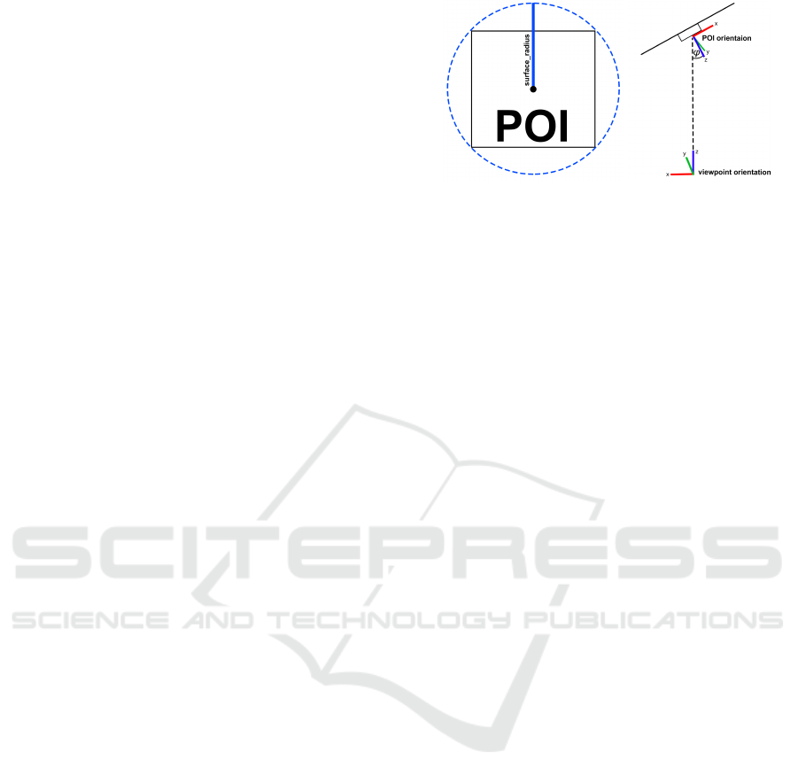
(a)
(b)
Figure 1: (a) Example POI with corresponding surface ra-
dius. (b) Deviation angle ϕ between the normal of the POI
and the optical axis of the camera.
3.3 Point of Interest
A Point-of-Interest, POI for short, is an individual
part or a low-order assembly on the component to
be inspected. POIs are described by its ID, position,
orientation, maximum deviation angle, semantic An-
notation and a surface radius. The position of the
POI in the workspace is indicated by its coordinates
x, y, z and its orientation x
q
, y
q
, z
q
, w
q
. The orientation
of the copter is defined over the division ring of the
quaternions H. The position specifies the center of
the POI. The maximum deviation angle ϕ
max
speci-
fies the maximum deviation of the angle ϕ between
the normal of the POI and the optical axis of the cam-
era, as shown in figure 1b. Each POI has a semantic
annotation that describes the low-order part or com-
ponent. To determine the camera position, the surface
radius is also needed. It describes the radius of the
POI on the surface of the part and is an approxima-
tion of the complex structure of the POI to a circle, as
shown in figure 1a.
3.4 Viewarea
A POI is visible to the UAVs camera from a certain
area, the so-called Viewarea. A Viewarea is calcu-
lated depending on the Angle-of-View (AoV) and the
focus of the camera, as well as the surface radius of
the POI to which the Viewarea is assigned. It is de-
scribed by the radii va
min
and va
max
. Where va
min
describes the minimum distance between the visual
sensor and the POI. It indicates the lower limit from
which a POI is no longer completely visible in the
image. However, if the required minimum distance to
the component is greater than this lower limit, va
min
represents the required minimum distance to the com-
ponent. The va
max
represents the upper limit, from
which on the POI is no longer visible in the picture.
Both parameters thus indicate a lower and upper limit
of the effectively usable viewarea.
Towards Fully Automated Inspection of Large Components with UAVs: Offline Path Planning
73

3.5 Viewpoint
Each POI has at least one viewpoint from which sen-
sor data can be collected. In the best case, it lies on the
inverted z-axis of the camera orientation, fixed at the
position of the POI. A viewpoint vp
i
that observes a
POI poi
j
with associated viewarea VA
j
is calculated
so that vp
i
∈ V P
i
. Here V P
i
contains all viewpoints
vp
i
in the following form:
V P
i
= {vp
i
∈ VA
j
: va
min
≤
||poi
j
− vp
i
||
2
≤ va
max
}
(1)
Furthermore, it can happen that two Viewareas are not
disjoint, i.e. there is a set A with Viewareas VA
i
⊇ V P
i
, VA
j
⊇ V P
j
and viewpoint vp
0
i
, so that the following
applies: A = {vp
0
i
: vp
0
i
∈ V P
i
∩V P
j
}. If A contains
viewpoints that maintain the maximum angle of de-
viation ϕ
max
for each POI they can theoretically ob-
serve, it is possible to use such sets A in the case of
optimizing the trajectory length between three adja-
cent viewpoints. A viewpoint is described by its ID,
position, orientation, a boolean parameter that indi-
cates whether the viewpoint lies in the middle of its
viewarea, three radii and a list of all POIs which it
observes. The position is given by the coordinates
x, y, z and the orientation by x
q
, y
q
, z
q
, w
q
. The orien-
tation of the viewpoints is defined above the division
ring of the quaternions H. Position and orientation
represent the position and orientation of the camera
lens relative to the origin of the coordinate space. If
the viewpoint cannot be optimally positioned (on the
inverted z-axis of the camera orientation fixed to the
position of the POI), the boolean parameter indicates
that it is an alternative viewpoint. The radii vp
min
and
vp
max
represent the effectively usable viewarea in the
xy-plane at the viewpoint position, depending on the
AoV of the camera. The radius r
ϕ
represents the ef-
fective viewarea in the xy-plane at the viewpoint po-
sition, depending on the deviation angle ϕ of the POI.
3.6 Key Viewpoint
If at least one viewpoint is found for each POI, the
number of viewpoints should be kept to a minimum.
As described in the previous paragraph, alternative
viewpoints can be calculated that can inspect more
than one POI. However, this may result in a worse
view on the POIs that vp
0
i
observes. Therefore, a
good trade-off between optimal viewpoint positions
and trajectory length must be found in the course of
optimization. In the end there should be at most one
viewpoint for each POI that observes it. The set of
these viewpoints are the so-called key viewpoints.
3.7 Trajectory
A UAV has so-called holonomic properties, i.e. its
controllable degree of freedom with respect to its
position corresponds to its total degree of freedom
with respect to its position. Therefore viewpoints can
be accessed directly and the trajectory between two
viewpoints can be described as a linear motion (LIN).
For this purpose, this paper assumes that there are no
obstacles between two adjacent viewpoints. Finally,
the trajectory contains a permutation of all key view-
points and represents a shortest route.
3.8 Planning of Viewpoints
Before the trajectory can be calculated, viewpoints
must be planned depending on the camera’s field of
view. The following section describes the require-
ments that need to be considered when planning view-
points and how viewpoints can be planned in detail:
3.8.1 Requirements for Viewpoint Planning
As stated by Alarcon et al. (Alarcon-Herrera et al.,
2014), a POI is optimally positioned in the image if
the optical axis of the camera runs along the normal
vector of the POI and a standoff-distance to the POI
is maintained (here: va
min
≤ stando f f distance ≤
va
max
). Since the tilt and inclination angle of the UAV
is not arbitrary selectable and the camera is statically
attached to the UAV, viewpoints have to be found so
that ϕ (see figure 1b) is within the given tolerance
range ϕ
max
and the standoff-distance is kept.
3.8.2 Planning
When planning a viewpoint, the radii of the viewarea
to a POI must be calculated and the orientation of the
camera must be taken into account. The minimum-
and maximum distance va
min
, va
max
between the
viewarea and a POI is calculated as follows:
va
min
=
poi
r
i
tan(
min(AoV )
2
)
(2)
va
max
= f ·
(poi
r
i
· φ)
2
[mm]
A
poi
[px]
(3)
Where f is the focal length of the camera, A
poi
the
minimum size of the POI in pixels in the picture so
that the POI can be identified and poi
r
i
the surface ra-
dius of Poi poi
i
. The constant φ indicates to which
extent A
poi
may be exhausted.
To examine the planning of the viewpoints under
ideal conditions first, the orientation of the POIs and
the camera was chosen so that the optical axis of the
ICINCO 2020 - 17th International Conference on Informatics in Control, Automation and Robotics
74
camera runs along the normal vector of the POI and
is therefore valid:
∀vp
i
, poi
i
(vp
i
, poi
i
) ∈ V P
i
× POI
i
⇒ ϕ = 0 (4)
Where POI
i
is the set of all POIs for a single part
or an assembly of lower order. V P
i
is the set as de-
scribed in Eq.1. If the z-axes of the camera, POI and
workspace are parallel to each other, the orientation
of the camera can be taken as the orientation of the
viewpoint. The position of the viewpoint is then a
translation around the standoff-distance along the z-
axis of the POI. Thus the POI is located on the optical
axis of the camera and the viewpoint is located in the
middle of the viewwarea. The radii of the Viewarea
at the position of the viewpoint are calculated as fol-
lows:
vp
max
(poi
i
, vp
j
) =
= tan(
max(AoV )
2
) · d(poi
i
, vp
j
) − poi
r
i
(5)
vp
min
(poi
i
, vp
j
) =
= tan(
min(AoV )
2
) · d(poi
i
, vp
j
) − poi
r
i
(6)
r
ϕ
(poi
i
, vp
j
) =
= tan(ϕ
max
) · d(poi
i
, vp
j
) − poi
r
i
(7)
d(poi
i
, vp
j
) = ||poi
i
− vp
j
||
2
(8)
The radii vp
min
and vp
max
are especially important if a
POI cannot be identified from a viewpoint during the
inspection. If a POI cannot be identified from a POI
during inspection, one of the radii can be used during
inspection to circle around the viewpoint in a spiral
flight. If the POI still cannot be identified, it will be
marked as not present.
3.9 Planning the Trajectory
After key viewpoints have been found for all POIs,
a trajectory containing all key viewpoints must be
planned. For this purpose, the following describes
which requirements have to be considered when plan-
ning a trajectory and how these can be fulfilled by
modelling the Travelings-Salesman-Problem as Ant
Colony Optimization.
3.9.1 Requirements for Trajectory Planning
For the offline planning of the trajectory there are
three main requirements: For each POI to be in-
spected, each key viewpoint must be located on the
trajectory. For easy handling of the UAV during the
inspection, the trajectory should end at the position
where it started. To minimize the time needed for the
inspection, the trajectory through all key-viewpoints
should be planned as short as possible.
3.9.2 Planning
The Ant Colony Optimization (ACO), a method for
solving the Travelings-Salesman-Problem, was used
to fulfill the requirements. This method is particularly
well suited for a large number of nodes (viewpoints)
because it provides a near-optimal solution (Chaud-
hari and Thakkar, 2019), as shown in table 1. Fur-
thermore, a near-optimal route can be found in a short
time by using ACO.
ACO is inspired by the behaviour of ants in find-
ing a shortest possible route from their nest to a food
source. For this purpose, ants leave pheromones on
their route when they have found a food source. Other
ants follow this pheromone trail with a certain prob-
ability, whereby the probability increases with the in-
tensity of the pheromone on the trail. After a certain
time, more and more ants follow the strongest/opti-
mal pheromone trail. Since more pheromones can be
deposited in the same time on a shorter route than on
a longer one, the intensity of the pheromone trace in-
creases most on the shorter route. Over time, the in-
tensity of the pheromone trace of less used routes de-
creases again.
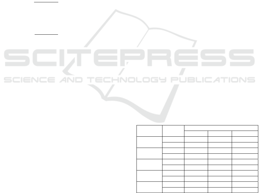
Table 1: Source: Chaudhari et al. (Chaudhari and Thakkar,
2019). Comparison of average and best found distances (in
km) of Ant Colony Optimization (ACO), Particle-Swarm-
Optimization (PSO), Artificial-Bee-Colony (ABC), Firefly
Algorithm (FA) and Genetic Algorithm (GA). Burma14 rep-
resents 14 cities in Burma, Bayg29 29 cities in Bavaria and
Att48 cities in the USA.
Algorithm Route
Few of the benchmark TSPs
Burma14 Bayg29 Att48
ACO
Average 31,05 9274,79 35043,34
Best 30,88 9195,22 34600,71
PSO
Average 32,34 15047,83 109979,87
Best 30,88 14036,75 91237,09
ABC
Average 32,36 17404,62 107883,76
Best 30,88 16658,30 101985,88
FA
Average 31,80 14283,51 81182,32
Best 30,88 13062,40 78479,69
GA
Average 31,49 11023,70 50753,50
Best 30,88 10018,10 46362,05
To imitate this behavior, first define the pheromone
update formula (Eq. 9) for each edge c
i j
in a graph
G = (V, E).
τ
i j
= (1 − ρ) · τ
i j
+
m
∑
k=1
∆τ
k
i j
(9)
Towards Fully Automated Inspection of Large Components with UAVs: Offline Path Planning
75

Where ρ is the pheromone evaporation rate, m the
number of ants and ∆τ
k
i j
(Eq. 10) the pheromone in-
tensity left by ant k at edge c
i j
.
∆τ
k
i j
=
Q
L
k
i f c
i j
is on the Route o f ant k
0 else
(10)
Where Q is a constant and L
k
is the route length of ant
k in the current iteration. The probability of taking the
edge c
i j
at node i to node j is given by Eq. 11.
p
k
i j
=
τ
α
i j
· η
β
i j
∑
c
il
∈N(s
p
)
τ
α
il
· η
β
il
i f c
i j
∈ N( j
p
)
0 otherwise
(11)
Where j
p
is the route taken by ant k so far and N( j
p
)
are the edges (i, l) to not yet visited nodes l. The pa-
rameters α, β control the influence of the pheromone
τ
i j
and the heuristic information η
i j
(Eq.12).
η
i j
=
1
d
i j
(12)
In this work the Ant Colony System (ACS) (Gam-
bardella and Dorigo, 1996; Stuetzle and Dorigo,
1999; Dorigo et al., 1999), a variation of the ACO,
was used. With ACS, only pheromone from the
globally best ant is deposited on an edge c
i j
and
the pheromone update formula changes to a Global
Pheromone Update Formula (Eq.13).
τ
i j
= (1 − ρ) · τ
i j
+ ρ · ∆τ
best
i j
(13)
Additionally, a local pheromone update formula (Eq.
14) is defined for each ant. This makes already visited
edges less interesting for other ants and increases the
exploration of not yet visited edges.
τ
i j
= (1 − ρ) · τ
i j
+ ρ · τ
0
(14)
τ
0
=
1
n · L
nn
(15)
Where n is the number of key viewpoints and L
nn
is
the length of a route according to the nearest neighbor
heuristic. In addition, formula (Eq. 11) is reformu-
lated to calculate the probability of which node will
be visited next by ant k. For this purpose, q ∈ [0, 1]
is randomly determined and q
0
is fixed as a constant.
The constant q
0
determines whether the focus should
be on the exploration of G or the exploitation of good
pheromone traces. Ant k then selects the next node j,
according to the formula (Eq. 16)
j =
argmax
c
i j
∈N( j
p
)
{τ
i j
· η
β
i j
} i f q ≤ q
0
J otherwise
(16)
p
k
i j
=
τ
i j
· η
β
i j
∑
c
il
∈N(s
p
)
τ
il
· η
β
il
i f c
i j
∈ N( j
p
)
0 otherwise
(17)
Here J is a random node j which has not yet been
visited by ant k and according to Eq. 17: This cal-
culation gives preference to nodes that are connected
to the current node i by a short edge and have a high
pheromone intensity.
The underlying graph G = (V, E) is a complete
graph, i.e. each key viewpoint is connected to each
by an edge. Since the trajectory consists of LINs be-
tween the key-viewpoints, the edge weights are equal
to the Euclidean distance between the key-viewpoints.
4 REALIZATION AND
IMPLEMENTATION
This chapter deals with the realization and implemen-
tation of the concept presented in chapter 3. For the
realization of the offline planning of the viewpoints
and the trajectory a software architecture was devel-
oped, which allows to define different requirements to
the viewpoint and trajectory planning and to extend
the system component by component. For trajectory
planning, it is shown how the Ant Colony System can
be implemented.
4.1 System Architecture
The elaboration of all presented concepts was ab-
stracted to a necessary level in order to first investigate
the suitability of UAVs for fully automated inspection
of given areas on the component. The design of the
system was therefore chosen in such a way that the
realization within the scope of this paper is limited
to the complete concept and can be extended beyond
that. For this reason, the software architecture placed
great emphasis on the scalability and interchangeabil-
ity of the viewpoint and trajectory planning compo-
nents with the aim of adapting the system to different
viewpoint and trajectory requirements. If, for exam-
ple, a trajectory is to be planned for multiple com-
ponents of the same type, a strategy can be selected
that keeps the length of the trajectory as short as pos-
sible, thus saving time and costs in visual inspection.
If, on the other hand, a trajectory is to be planned for
individual components, a much less computationally
intensive strategy can be used to plan the trajectory if
a fast calculation of the trajectory is essential. In or-
der to plan viewpoints and trajectory, camera parame-
ters, minimum distance of the UAV to the component
ICINCO 2020 - 17th International Conference on Informatics in Control, Automation and Robotics
76

and the desired planning strategy are transferred to the
system. The camera parameters necessary for the sys-
tem are the orientation of the camera lens relative to
the orientation of the UAV, angle of view, focal length
and the desired minimum size of a POI in the image
in pixels. The strategy for viewpoint and trajectory
planning is then instantiated via an abstract factory.
Which factory should be used is determined by the
implementation of the strategy pattern: The strategy
for viewpoint planning is determined using the trans-
ferred parameters and the corresponding factory is se-
lected. If a new strategy is to be added to the system, a
new factory can be added by implementing the corre-
sponding interface. The system outputs the trajectory
and the key viewpoints in serialized form. Afterwards
the planned trajectory can be tested simulatively with
ROS, Gazebo and Rviz or the key viewpoints can be
sent to a UAV via mavlink.
4.2 Viewpoint and Trajectory Planning
The viewpoint and trajectory planning component
were realized and implemented in Python 3. The ex-
act elaboration is described below.
4.2.1 Viewpoint Planning
When planning the viewpoints, the radii were calcu-
lated according to the formulas in chapter 3.8.2. To
calculate the position of the viewpoint, the x and y
position of the POI was taken and the position of the
viewpoint along the z-axis of the POI was shifted by
the va max radius of the associated viewarea. The
va max radius distance between the viewpoint and
the POI was chosen to allow the UAV to initially
maintain a certain safety distance to the component.
The orientation of the camera has been adopted as
the viewpoint orientation. This is possible for the
case under consideration because the z-axis of the
workspace, the optical axis of the camera and the nor-
mal of the POI are parallel to each other.
4.2.2 Trajectory Planning
The implementation of the ACS is based on the con-
cept of Trevlovett (trevlovett, ). The implementation
of the ACS is multithreaded, i.e. each ant was imple-
mented as a single thread. The distance between the
key viewpoints and the pheromone intensity on the
edges are created as two separate matrices. The Eu-
clidean distance between the key-viewpoints is used
as the distance measure, since the trajectory is defined
as LINs between the key-viewpoints. The pheromone
intensity on each edge is initially set to τ
0
:
τ
0
=
1
1
2N
·
∑
c
i j
||i − j||
2
(18)
where N is the number of key viewpoints. The calcu-
lation of the global and local pheromone update for-
mula was done as in Eq. 13 and Eq. 14 and the heuris-
tic information η
i j
as in Eq. 12. The formula for the
pheromone intensity at edge c
i j
was calculated as fol-
lows:
∆τ
best
i j
=
||i − j||
best
2
L
best
k
(19)
Where ||i − j|||
best
2
is the Euclidean distance of the
edge c
i j
on the best route and L
best
k
is the distance of
the best route.
The implementation of the formula as in Eq. 17, was
implemented as a roulette wheel-style selection pro-
cedure. This is done by taking the average value of
the pheromone and heuristic information of all edges
c
il
∈ N( j
p
):
avg =
∑
c
il
∈N(s
p
)
τ
il
· η
β
il
N
R
(20)
Where N
R
is the number of viewpoints not yet visited.
The edge to the first viewpoint in the list of unvisited
viewpoints whose pheromone and heuristic informa-
tion value of the edge is greater than avg is taken. The
implementation is based on the ROS infrastructure
and can be visualized with Rviz. Gazebo was used
to simulate the behavior of the UAVs and the visual
sensors. For illustrative purposes we provide videos
of the implementation of the simulation environment
as well as the processing of the trajectory (ros, ; rvi, ).
5 EVALUATION
For the evaluation, nine POIs were considered, which
are attached to a component. The orientation of the
POIs were chosen so that their normals are parallel to
the z-axis of the workspace. For the additional evalu-
ation of the trajectory planning, the results of the im-
plementation were evaluated using a TSP-benchmark
data set. The trajectory through the nine key view-
points was tested with Gazebo, Rviz and ROS. The
results of the evaluation are shown below.
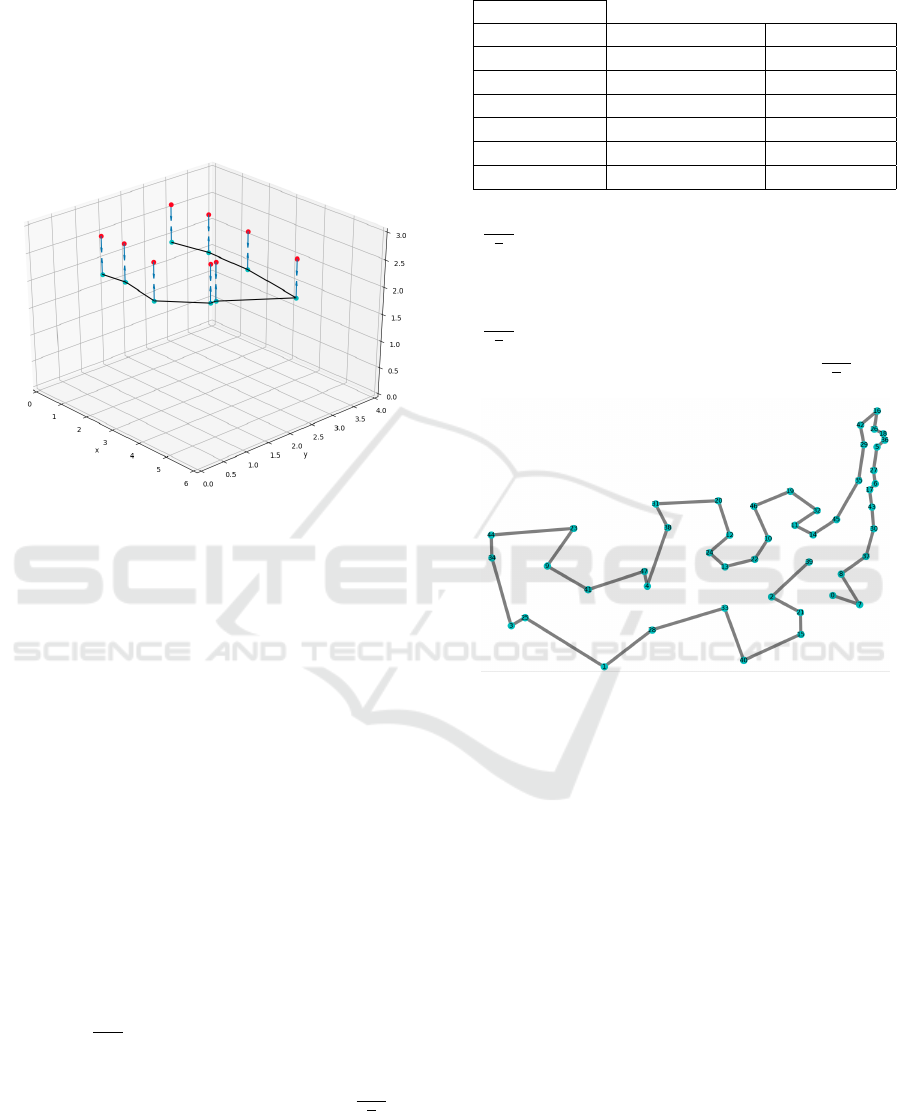
5.1 Results of Trajectory Planning
As described in chapter 3.9, the trajectory is planned
in a complete graph G = (V, E). For each of the nine
POIs, a viewpoint has been planned which is located
in the middle of the POI’s Viewarea. The optical axis
of the camera is always on the normal of the POI, so
Towards Fully Automated Inspection of Large Components with UAVs: Offline Path Planning
77
that for all pairs (vp
i
, poi
i
) ∈ V P
i
×POI
i
the deviation
angle ϕ is 0. An almost optimal route of 11.78 me-
ters through all nine key viewpoints was found after
twenty iterations of the procedure described in section
4.2.2. The found route in G, as well as the course of
the route through all key viewpoints including the as-
sociated POIs, their normals and the z-orientation of
the key viewpoints can be seen in figure 2.
Figure 2: Planned trajectory through all key viewpoints to
their corresponding POIs. The vectors of the POIs corre-
spond to the z-orientation and those of the viewpoints to the
optical axis of the camera.
5.1.1 Evaluation of the ACS Implementation
The implementation of the ACS was evaluated on the
Att48 benchmark dataset. (att, ) Att48 consists of the
distance relationships between 48 cities in the USA.
For the number of ants, as well for the parameters β
and ρ the results of the work of Pettersson et al. (Pet-
tersson and Lundell Johansson, 2018) are used:
β = 5, ρ = 0, 5, m = b0, 3 · Nc (21)
Where m is the number of ants and N is the number
of key viewpoints. The implementation was evaluated
using the Att48 dataset and it was examined which
ratio of ants to iterations yields a good trade-off of
found distance to required computing time. The num-
ber of iterations was calculated based on the num-
ber of ants, which in turn, as in Eq. 21, depends
on the number of key viewpoints. For this purpose,
the value b
2000
m
c by Pettersson et al. (Pettersson and
Lundell Johansson, 2018) were used and examined to
what extent better results can be achieved by increas-
ing the number of iterations. The values b
2000
m
i
c for
i ∈ {2, 3, 4, 5, 6, 7} were tested. With each value, ten
passes were performed. The average result for each
value can be seen in Table 2. The best distance on
the Att48 record of 34023.35 km was achieved with
Table 2: Comparison of the results with different choice of
iterations.
Att48
iterations ∅ lenght [in km] ∅ time [in s.]
2000 / (m / 2) 36483.416 84.262
2000 / (m / 3) 35937.116 124.487
2000 / (m / 4) 36261.336 173.377
2000 / (m / 5) 36031.142 217.897
2000 / (m / 6) 36061.551 247.518
2000 / (m / 7) 35929.504 293.229
b
2000
m
7
c iterations. This result undercuts the result ob-
tained by Chaudhari et al. The course of the best dis-
tance found in this work on the Att48 data set is shown
in figure Although the best results were obtained with
b
2000
m
7
c iterations, no significant better results were ob-
tained by increasing the iterations beyond b
2000
m
2
c.
Figure 3: Course of the route for the distance of 34023.35
km.
5.2 Results in Simulation
To check the trajectory in the simulation, the trajec-
tory, consisting of the nine key viewpoints, was trans-
ferred to the ROS node. As can be seen in figure 4,
the trajectory could be followed through the nine key
viewpoints. Here it can be observed that the move-
ment between the key viewpoints is not always linear.
The exact reason for this is unknown, but it is most
likely due to the local-planner, which requires sev-
eral attempts to get to the viewpoint using Adaptive
Monte Carlo Localization. Another reason could be
the defined speed of the UAV. It was observed that the
higher the speed was defined, the longer it took the
UAV to reach a viewpoint. Since the deceleration be-
havior of the UAV was not defined near a viewpoint,
it is possible that the UAV flies over viewpoints, then
decelerates and tries to reach the viewpoint again.
This procedure may be repeated several times.
ICINCO 2020 - 17th International Conference on Informatics in Control, Automation and Robotics
78
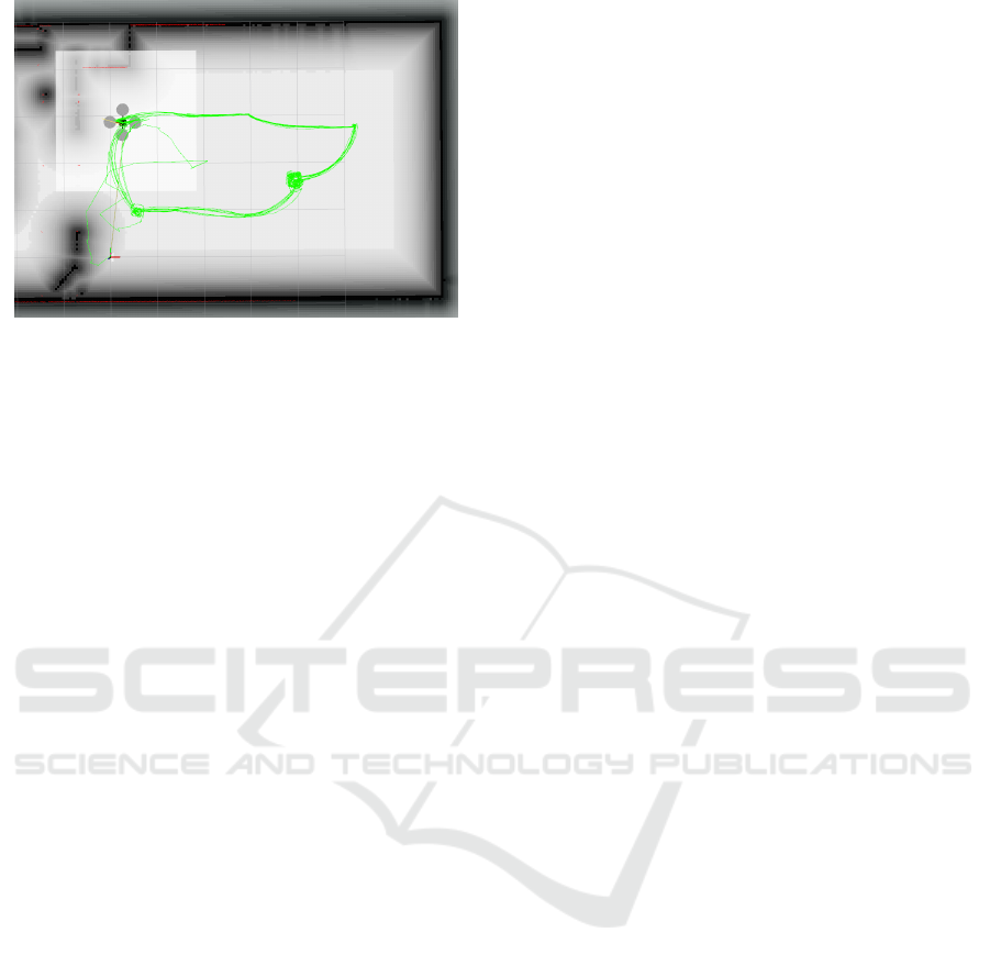
Figure 4: Performed trajectory in the simulation.
6 CONCLUSION AND FUTURE
WORK
Within the scope of this paper the feasibility of offline
trajectory planning for fully automated visual inspec-
tion of predefined areas on a component was inves-
tigated. It was shown how viewpoints to predefined
parts on the component can be planned and what has
to be considered during the planning. The planning of
viewpoints was examined for the use of UAVs. Fur-
thermore, it was shown how the Ant-Colony-System
can be used to plan a trajectory that contains all key-
viewpoints and can be planned in short time and has
a nearly optimal length. However, a number of mile-
stones still need to be reached before fully automated
visual inspection can be performed by UAVs for large
components:
First of all, the planning of optimal viewpoints
of any orientation of the POIs has to be more inves-
tigated.If the maximum deviation radius allows the
viewpoint to be off the optical axis, it is important
to check how to plan viewpoints that observe multi-
ple POIs simultaneously and shorten the overall tra-
jectory length. Furthermore, it must be possible for
the system to evaluate viewpoints that have already
been found offline: First of all, it must be checked
whether a viewpoint is located in the area of a static
obstacle on the component, whether the field of view
on the POI is blocked by a static obstacle or whether
the viewpoint is otherwise not accessible by the UAV.
Also, light conditions and shading can make it dif-
ficult to inspect a POI. It is therefore necessary to
investigate how to take into account difficult inspec-
tion conditions when planning offline and how to plan
viewpoints so that difficult conditions can be dealt
with more easily during the inspection.
In section 3.8, a strategy was presented for how
to proceed if a POI cannot be identified from a view-
point during the inspection. However, this is only one
way to deal with such a situation. It is also possible
to consider procedures that already plan and provide
alternative viewpoints to a POI offline. Furthermore,
when inspecting predefined areas of the component,
the Coverage Planning must also be considered. This
is necessary if geometrically complex and/or large
POIs on the part are to be inspected and a single view-
point per POI is no longer sufficient.
The existence check examined in this paper is only
one use case for the inspection of predefined areas on
the component. Further use cases, which have to be
investigated in the future, are the relative orientation
of a POI in the component, as well as the attachment
of the POI to the component.
There are also areas of trajectory planning that can
be optimized. As in viewpoint planning, obstacles
must also be taken into account when planning the
trajectory. Therefore it must be possible to check in
the context of trajectory planning whether adjoining
key viewpoints can be reached by a linear trajectory
of the UAV and how the obstacles between adjoining
key viewpoints can be avoided. Another point of opti-
mization is the current view of the trajectory as LINs
between the key viewpoints. Depending on the in-
spection scenario, point-to-point or trajectory control
could also be considered.
The automated visual inspection of large compo-
nents by UAVs is still in its infancy, but it is a nec-
essary step to make visual inspections of components
more precise, easier and more efficient in the future.
REFERENCES
Localization using laser-based slam. last access: 29.03.20.
Mp-testdata - the tsplib symmetric traveling salesman prob-
lem instances. last access: 25.04.20.
Trajectory trough all viewpoints. last access: 29.03.20.
Alarcon-Herrera, J. L., Chen, X., and Zhang, X. (2014).
Viewpoint selection for vision systems in industrial in-
spection. In 2014 IEEE International Conference on
Robotics and Automation (ICRA), pages 4934–4939.
Bircher, A., Alexis, K., Burri, M., Oettershagen, P., Omari,
S., Mantel, T., and Siegwart, R. (2015). Structural in-
spection path planning via iterative viewpoint resam-
pling with application to aerial robotics. In 2015 IEEE
International Conference on Robotics and Automation
(ICRA), pages 6423–6430.
Chaudhari, K. and Thakkar, A. (2019). Travelling salesman
problem: An empirical comparison between aco, pso,
abc, fa and ga. In Shetty, N. R., Patnaik, L. M., Na-
garaj, H. C., Hamsavath, P. N., and Nalini, N., editors,
Emerging Research in Computing, Information, Com-
munication and Applications, pages 397–405, Singa-
pore. Springer Singapore.
Towards Fully Automated Inspection of Large Components with UAVs: Offline Path Planning
79

Danner, T. and Kavraki, L. E. (2000). Randomized planning
for short inspection paths. In Proceedings 2000 ICRA.
Millennium Conference. IEEE International Confer-
ence on Robotics and Automation. Symposia Proceed-
ings (Cat. No.00CH37065), volume 2, pages 971–976
vol.2.
Deutsche Bahn AG (2020). Kompetenzcenter Multicopter
DB.
Dorigo, M., Caro, G. A. D., and Gambardella, L. M. (1999).
Ant algorithms for discrete optimization. Artificial
Life, 5:137–172.
Englot, B. and S. Hover, F. (2014). Sampling-based cov-
erage path planning for inspection of complex struc-
tures. ICAPS 2012 - Proceedings of the 22nd In-
ternational Conference on Automated Planning and
Scheduling.
Galceran, E. and Carreras, M. (2013). A survey on coverage
path planning for robotics. Robotics and Autonomous
Systems, 61:1258–1276.
Gambardella, L. M. and Dorigo, M. (1996). Solving sym-
metric and asymmetric tsps by ant colonies. In Pro-
ceedings of IEEE International Conference on Evolu-
tionary Computation, pages 622–627.
Gonz
´
alez-Banos, H. (2001). A randomized art-gallery al-
gorithm for sensor placement. Proc. 17th ACM Symp.
Comp. Geom., pages 232–240.
Jordan, S., Moore, J., Hovet, S., Box, J., Perry, J., Kirsche,
K., Lewis, D., and Tse, Z. T. H. (2018). State-of-the-
art technologies for uav inspections. IET Radar, Sonar
Navigation, 12(2):151–164.
Karaman, S. and Frazzoli, E. (2011). Sampling-based algo-
rithms for optimal motion planning. The International
Journal of Robotics Research, 30(7):846–894.
Laporte, G. (1992). The traveling salesman problem: An
overview of exact and approximate algorithms. Euro-
pean Journal of Operational Research, 59:231–247.
LaValle, S. M. (2006). Planning Algorithms. Cambridge
University Press.
Malandrakis, K., Savvaris, A., Domingo, J. A. G., Avde-
lidis, N., Tsilivis, P., Plumacker, F., Fragonara, L. Z.,
and Tsourdos, A. (2018). Inspection of aircraft wing
panels using unmanned aerial vehicles. In 2018
5th IEEE International Workshop on Metrology for
AeroSpace (MetroAeroSpace), pages 56–61.
O’Rourke, J. (1987). Art Gallery Theorems and Algorithms.
Oxford University Press, Inc., New York, NY, USA.
Pettersson, L. and Lundell Johansson, C. (2018). Ant
colony optimization - optimal number of ants.
Stuetzle, T. and Dorigo, M. (1999). Aco algorithms for the
traveling salesman problem.
trevlovett. Python ant colony tsp solver. last access:
10.10.2019.
ICINCO 2020 - 17th International Conference on Informatics in Control, Automation and Robotics
80
