
Approaches to Parameter Identification for
Hybrid Multilinear Time Invariant Systems
Aadithyan Sridharan
1 a
, Gerwald Lichtenberg
1 b
, Antonio Correcher Salvador
2 c
and Carlos Vargas Salgado
3 d
1
Faculty of Life Sciences, University of Applied Sciences, Ulmenliet 20, 21033 Hamburg, Germany
2
Instituto Universitario de Autom
´
atica e Inform
´
atica Industrial (ai2),
Universitat Polit
`
ecnica de Val
`
encia, 46022, Valencia, Spain
3
Department of Electrical Engineering, Universitat Polit
`
ecnica de Val
`
encia, 46022, Valencia, Spain
Keywords:
Multilinear Systems, Parameter Identification, Tensor Decomposition, Industrial Building Modelling.
Abstract:
Industrial buildings often have interacting continuous- and discrete-valued signals. Hybrid multilinear time
invariant (MTI) models have been shown to be able to describe this hybrid dynamics appropriately for many
cases. White box modelling methods from first principles have been used in this application domain before.
The parameters of these models can be efficiently represented by higher order tensors. This paper introduces
as alternatives black and grey box approaches for the parameter identification of MTI models from data. The
methods are tested with the help of simulation data produced from a multilinear model of an industrial hall. It
is assumed that all state variables are measured with additative noise and the input and disturbances are exactly
measured, too. Two black box methods obtain either the full parameter tensor or a rank-r decomposition of it.
Numerical examples using the industrial building model show the principle applicability of these approaches
for real data.
1 INTRODUCTION
Systems in many application areas as buildings engi-
neering show discrete-valued as well as continuous-
valued signals, e.g. if a continuous state like a temper-
ature depends on the switching ON/OFF of a binary
input like a gas heater. This example can be suffi-
ciently good described by multilinear time invariant
(MTI) models, as well as many more from other ap-
plication areas, (Lichtenberg, 2011).
There are three traditional approaches in order to
obtain a state space model depending on the avail-
able information about the system. If no sufficient
prior knowledge about the system is available, then
the black box identification approach is chosen (Cha-
van and Talange, 2018), (Tayamon, Zambrano, Wi-
gren and Carlsson, 2011), (Royer, Thil, Talbert and
Polit, 2014). On the contrary, in some cases through
first principles like laws of physics, sufficient infor-
a
https://orcid.org/0000-0002-1237-3125
b
https://orcid.org/0000-0001-6032-0733
c
https://orcid.org/0000-0002-2443-9857
d
https://orcid.org/0000-0002-9259-8374
mation about the system can be obtained. In these
cases, white box techniques are used. However, if the
information through first principles is incomplete, in
the sense that there are unknown parameters in the
system, the grey box identification approach is used
(Bacher and Madsen, 2011).
In (Batselier, Ko, Phan, Cichoki and Wong, 2018),
the system identification problem of multilinear state
space models has been considered. In this work, the
coefficients of the state space matrices have been es-
timated by representing them as tensor train matrices.
The computational complexity is reduced by repre-
sentation as tensor train matrices. The contribution of
this paper are different methods for parameter identi-
fication of an MTI state space model. In order to solve
the identification problem, both the grey and black
box methods are considered. The grey box problem
involves finding the unknown physical parameters of
the system. In this case the structure of the model is
known beforehand.
On the other hand, the black box problem involves
no prior knowledge about the system. The identifi-
cation problem is to find parameters of a multilinear
state space model, given a set of input state data and
Sridharan, A., Lichtenberg, G., Salvador, A. and Salgado, C.
Approaches to Parameter Identification for Hybrid Multilinear Time Invariant Systems.
DOI: 10.5220/0009887502550262
In Proceedings of the 10th International Conference on Simulation and Modeling Methodologies, Technologies and Applications (SIMULTECH 2020), pages 255-262
ISBN: 978-989-758-444-2
Copyright
c
2020 by SCITEPRESS – Science and Technology Publications, Lda. All rights reserved
255
a specific system order. The first black box method
shows how the parameter identification problem can
be transformed to a linear least squares problem and
thus solved efficiently. The parameters of the MTI
state space model increase exponentially with respect
to the order of the system and the number of inputs.
As the parameters of MTI state space models can nat-
urally be represented as tensors, decomposition meth-
ods can be used to compute low rank approximations,
which need only a remarkable less number of param-
eters, especially for the case of canonical polyadic
(CP) decompositions, (Kruppa, 2017). The second
approach to black box parameter identification given
in this paper is a direct estimation method for the CP
decomposition factors of the parameter tensor from
data. Throughout the paper, discrete time models are
used and the inputs as well as state signals are as-
sumed to be sampled with a fixed sampling time. The
effects of measurement noise are not dealt with by a
formal approach. However, simulation results are pre-
sented by adding noise as well.
The paper is organized as follows. Firstly, a brief
introduction to tensor calculus and MTI systems is
given. Thereafter, the identification problem is setup
and is dealt with by the methods described above. Fi-
nally, a numerical example simulated using MATLAB
Simulink is presented, followed by conclusion and fu-
ture scope.
2 TENSOR BASICS
The state space model of an MTI system can be for-
mulated in a tensor framework. Thereby, in this sec-
tion, some basic concepts about tensors and tensor de-
compositions are presented (Kolda and Bader, 2009).
Definition 1 (Tensor). A multidimensional n-way ar-
ray
X ∈ R
I
1
×I
2
×···×I
n
(1)
where (I
1
, I
2
, ..., I
n
) ∈ N
n
is called a real tensor of or-
der n.
Although such a structure can store complex val-
ues as well, in the current work, only real values are
dealt with. An element
x(i) = x(i
1
, i
2
, ..., i
n
) ∈ R
of the tensor X can be selected by the index vector
i = (i
1
, i
2
, ..., i
n
).
For tensors, numerous arithmetic operations exist
and two of them are used in this paper: the contracted
product of two tensors A, B is denoted by h A |B i
whereas the outer product is denoted by A ◦ B. In
depth information on these products can be found in
(Kolda and Bader, 2009).
Tensors can have very high storage demands,
since the number of elements of a tensor depends
exponentially on the number of dimensions of the
tensor. In order to address this problem, tensor de-
composition methods have been developed over the
last decades, (Cichocki, Zdunek, Phan and Amari,
2009). Decomposition methods range from canoni-
cal polyadic (CP), Tucker, tensor trains to hierarchi-
cal decompositions. Because of their superior storage
effort savings and suitability to MTI models, CP de-
compositions are used in this paper. The simplest of
it is given in the next definition.
Definition 2 (Rank One Tensor). An n dimensional
tensor
X = x
1
◦ x
2
◦ ··· ◦ x
n
∈ R
I
1
×I
2
×···×I
n
(2)
has rank one if it can be computed by the outer prod-
uct of n vectors x
i
∈ R
I
i
∀i = 1, ..., n.
All full tensors are representable by a sum of rank
one tensors, which is given in the next definition.
Definition 3 (CP Tensor). A canonical polyadic rep-
resentation
K = [X
1
, X
2
, ..., X
N
] · λ (3)
=
r
∑
l=1
λ(l)x
1
(:, l)◦ ·· · ◦ x
N
(:, l) (4)
of a real tensor of dimension I
1
× I
2
× ··· × I
n
is given
by a sum of rank 1 tensors.
The elements are computed by the sums of
the outer products of the column vectors of fac-
tor matrices X
i
∈ R
I
i
×r
. The introduction of a
weighting vector λ ∈ R
r
allows to normalize the
column vectors of the factor matrices. The minimum
number of rank 1 tensors required to reproduce the
original tensor K is called the CP rank of the tensor K.
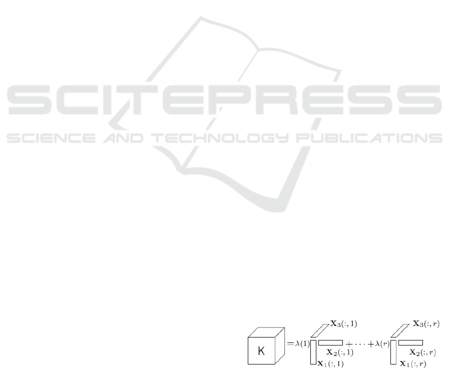
Example 1. Figure 1 visualizes a 3rd order CP ten-
sor
K = [X
1
, X
2
, X
3
] · λ
=
r
∑
l=1
λ(l)X
1
(:, l)◦ X
2
(:, l)◦ X
3
(:, l)
Figure 1: CP tensor (Kruppa and Lichtenberg, 2017).
SIMULTECH 2020 - 10th International Conference on Simulation and Modeling Methodologies, Technologies and Applications
256

3 MULTILINEAR MODELS
MTI systems are described by multilinear functions
depending on states and inputs. Multilinearity means
that the function is linear if all but one variables are
held constant. Thus, they are polynomials of order n
but showing a maximum order of one for each vari-
able, (Pangalos, Eichler and Lichtenberg, 2015).
Definition 4 (Multilinear Function). The function
f (x) = α
T
m(x) (5)
where
α =
α
1
·· · α
2
n
T
∈ R
2
n
is a coefficient row vector and
m(x) =
1
x
n
⊗ ··· ⊗
1
x
1
∈ R
2
n
is a column vector of monomial is called multilinear.
Here, ⊗ is the well known Kronecker product.
Definition 5 (MTI Matrix Model). A discrete-time
multilinear model is represented by a next state equa-
tion
x(k + 1) = F · m(x(k), u(k)) (6)
where m(x(k), u(k)) is given by
1
u
m
(k)
⊗·· ·⊗
1
u
1
(k)
⊗
1
x
n
(k)
⊗·· ·⊗
1
x
1
(k)
i.e. the monomial vector containing all multiplicative
combinations of states and inputs at time k.
The transition matrix F ∈ R
n×2
n+m
holds the
parameters of the model as the following example
shows.
Example 2. A MTI state space model of order two
x
1
(k + 1) = f
11
+ f
12
x
1
(k) + f
13
x
2
(k) + f
14
x
1
(k)x
2
(k)
x
2
(k + 1) = f
21
+ f
22
x
1
(k) + f
23
x
2
(k) + f
24
x
1
(k)x
2
(k)
has a transition matrix and monomial vector given by
F =
f
11
f
12
f
13
f
14
f
21
f
22
f
23
f
24
,
m(x
1
(k), x
2
(k)) =
1
x
1
(k)
x
2
(k)
x
2
(k)x
1
(k)
.
Next, the multilinear structure of the functions can be
exploited to represent the next state equation in a ten-
sor format.
Definition 6 (MTI Tensor Model). The next state
equation (6) can equivalently be written by
x(k + 1) = hF |M(x(k), u(k))i (7)
where F ∈ R
×
(n+m)
2×n
contains the parameters of the
model arranged as a tensor and M(x, u) ∈ R
×
(n+m)
2
is
a monomial tensor. The notation ×
(n+m)
2 stands for
2 × 2 × ... × 2
|
{z }
(n+m)times
.
Example 3. An autonomous MTI state space model
of order two in tensor form is given by
x
1
(k + 1)
x
2
(k + 1)
= h F | M(x
1
(k), x
2
(k)) i .
For this example, the contracted product of the tran-
sition tensor F ∈ R
2×2×2
and the monomial tensor
M ∈ R
2×2
leads to the same next state equations as
in the matrix case of Example 2.
The monomial tensor is already rank one and thus,
minimal. The parameter tensor can be decomposed as
CP tensor
F = [F
u
m
, .., F
u
1
, F
x
n
, .., F
x
1
, F
Φ
] · λ
F
(8)
which is e.g. discussed in (Pangalos, 2016).
With the parameter tensor (8), the next state equa-
tion (7) can be simplified
x(k + 1) = F
Φ
λ
F
~ F
T
u
m
1
u
m
(k)
~ ···~
~F
T
u
1
1
u
1
(k)
~ F
T
x
n
1
x
n
(k)
~ · ··~ F
T
x
1
1
x
1
(k)
!
(9)
The element wise multiplication, also known as the
Hadamard product is denoted as ~ operation and ma-
trix vector multiplication has precedence here.
Example 4. The previous example in decomposed
tensor representation has the next state equation
x(k + 1) = F
Φ
λ
F
~ F
T
x
2
1
x
2
(k)
~
~F
T
x
1
1
x
1
(k)
!
(10)
the weighting vector
λ
F
=
f
11
. . . f
14
f
21
. . . f
24
T
Approaches to Parameter Identification for Hybrid Multilinear Time Invariant Systems
257

and the factor matrices
F
Φ
=
1 1 1 1 0 0 0 0
0 0 0 0 1 1 1 1
F
x
1
=
1 0 1 0 1 0 1 0
0 1 0 1 0 1 0 1
F
x
2
=
1 1 0 0 1 1 0 0
0 0 1 1 0 0 1 1
4 IDENTIFICATION PROBLEM
In this section, the identification problem is formu-
lated for both grey and black box methods. Within
black box identification, the problem is tackled by two
different approaches.
4.1 Grey Box Identification
In this sub-section, it is assumed that a model from the
laws of physics is already available, albeit with un-
known parameters. Considering the following model
with n states, m inputs and l disturbances in discrete
time domain
x
1
(k + 1)
.
.
.
x
n
(k + 1)
=
f
11
+ f
12
x
1
(k) + .. + f
12
n+m+l
n
∏
i=1
x
i
m
∏
i=1
u
i
l
∏
i=1
d
i
.
.
.
f
n1
+ f
n2
x
1
(k) + .. + f
n2
n+m+l
n
∏
i=1
x
i
m
∏
i=1
u
i
l
∏
i=1
d
i
(11)
The discrete time MTI state space model for the
system in (11) is of order n with state vector x ∈ R
n
,
having an input vector u ∈ R
m
inputs and disturbances
d ∈ R
l
.
x(k + 1) = Fm (x(k), u(k), d(k)) (12)
where F ∈ R
n×2
n+m+l
is the matrix containing the
parameters ( f
11
, .., f
n2
n+m+l
) of the MTI state space
model. m(x(k), u(k), d(k)) is the monomial vector as
already introduced in section 3.
Assuming that the states of the MTI state space
model in (12) can be measured, then the parameter es-
timation problem can be formulated as, given an ini-
tial state x(0), a set of inputs u(k), set of disturbance
inputs d(k) and a set of real measured data
˜
x(k) where
k = 0, 1, .., T , find the parameter matrix F containing
the parameters ( f
11
, .., f
n2
n+m+l
) in the sense that the
sum J of squared errors e is minimum.
min
F
J (13)
J =
1
2
(e
T
Qe) (14)
where Q ∈ R
nT ×nT
is a diagonal, positive semi def-
inite weighting matrix for normalization of the mea-
sured signals.
Q = diag(q
1
, q
2
, .., q
nT
)
e =
x(1) −
˜
x(1)
.
.
.
x(T ) −
˜
x(T )
(15)
For i = 1..T , the states x(i) are the one step ahead
predictions from the model (12) using the measured
states
˜
x(i−1), the inputs u(i−1) and the disturbances
d(i − 1) in the previous time step. The objective is
to find the parameters set that minimizes the error
between the measured state
˜
x(i) and predicted state
x(i) from the MTI model in (12). The assumption
is that the parameters are constants and not varying
with time. The parameter matrix can be determined
in a straight forward way by simply solving an inverse
problem. Considering the MTI state space model in
matrix form introduced in the equation (12). Given
the data-set (
˜
x(k), u(k), d(k) for all k = 0, 1, .., T ), for
a model order n, with m inputs and l disturbances
˜
X = F · M (16)
where
˜
X ∈ R
n×T
, F ∈ R
n×2
n+m+l
and M ∈ R
2
n+m+l
×T
.
˜
X
T
=
˜
x(1)
˜
x(2)
.
.
.
˜
x(T )
(17)
M
T
=
m(x(0), u(0), d(0))
m(x(1), u(1), d(1))
.
.
.
m(x(T − 1), u(T − 1), d(T − 1))
(18)
Assuming T is large enough such that the given sys-
tem of equations is over-determined, the solution is:
F =
˜
X · M
−1
(19)
Solving the equation (19) will also minimize the sum
of squared errors as mentioned in (13).
4.2 Black Box Identification
For this case, no prior knowledge about the system
is available from the laws of physics. Thereby, the
problem now is to find a state space model of order n,
from a given a input-state data set, instead of finding
the unknown physical parameters of the system.
We solve the problem in two ways. First, the pa-
rameter matrix F is calculated by solving an inverse
problem. Thereafter, as shown in the section 3, MTI
state space model can be written in tensor form as well
and hence, the problem is solved by calculating the
CP factors of the parameter tensor F.
SIMULTECH 2020 - 10th International Conference on Simulation and Modeling Methodologies, Technologies and Applications
258
4.2.1 Inverse Problem
The inverse problem approach is similar to the solu-
tion discussed for the grey box problem in the equa-
tion (19). It follows from the solution in (19) that, for
a solution to exist, MM
T
must be non-singular and
thereby, full rank. For this to have full rank, all the
dynamic modes of the system must be excited. Since
the only set of influence-able variables of the T sam-
ple monomial matrix are the inputs, they must be rich
enough to excite all the modes of the system. This
is the well known concept of persistence excitation
(Ljung, 1999).
4.2.2 Estimation of Tensor Factors
In (7), it is shown how an MTI state space model can
be written in tensor form and thereafter, in (8) the CP
decomposed form of the tensor model is shown. The
objective here is to estimate the CP factors of the pa-
rameter tensor directly from the measurements. As-
suming a rank r CPD of the parameter tensor F such
that
F = [F
u
m
, .., F
u
1
, F
x
n
, .., F
x
1
, F
Φ
] · λ
F
(20)
where all of F
u
m
, .., F
u
1
, F
x
n
, .., F
x
1
∈ R
2×r
, F
Φ
∈ R
n×r
and λ
F
∈ R
r
.
The one step ahead predicted states x(k) as shown
in the error vector in (15) can be calculated from (9).
Using the error vector in (15), the least squares op-
timization problem in (13) can be solved for the un-
known factors of the parameter tensor. The optimiza-
tion problem is:
min
F
u
m
,..,F
u
1
,F
x
n
,..,F
x
1
,F
Φ
,λ
F
J (21)
The problem (21) turns out to be a nonlinear opti-
mization problem. Solutions to such problems can
be found by using the nonlinear optimization solvers
in the simulation environment of MATLAB Simulink.
An important variable in the given problem is the as-
sumed rank r of the CPD. The more the multilinear
terms present to calculate the state in the next time
step, the denser the parameter tensor becomes and
thereby, the CP rank of the parameter tensor also in-
creases. Hence, while choosing the rank of the CPD
one must consider that there is a trade off between the
savings in storage effort and the accuracy of the de-
composed tensor with respect to the original tensor.
5 APPLICATION
In this section, the simulation results of the MTI state
space model identification are presented. The identi-
fication will be performed for the heating system of
an industrial building.
5.1 Heating System
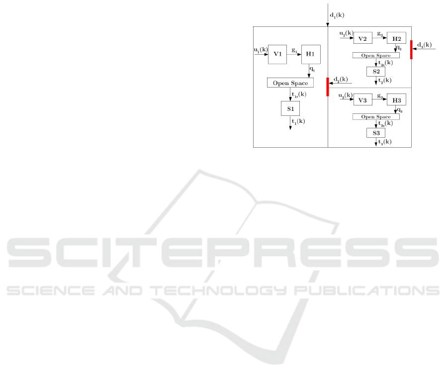
Figure 2: Heating system.
In figure 2, the schematic diagram of the heating sys-
tem of three heat zones of an industrial building is
clearly shown. Each heat zone has one heating device
which is a gas heater denoted by Hi, i=1..3. Depend-
ing on the input u
i
(k) ∈ E, i = 1..3, where E ∈ {0, 1, 2}
to the valves Vi, i=1..3, a volume of gas g
i
, i = 1..3
goes into the gas heater. The gas heater emits heat
flow q
i
, i = 1..3, depending on the gas inlet. Natu-
rally, the heat flow causes changes in the temperature
t
i
(k) ∈ R, i = 1..3 of the zone. The absolute temper-
ature of each the zones is measured by the respective
sensors Si, i=1..3. Additionally, there are three exter-
nal influences on the heating system as well. Two of
the three influences (d
2
(k) and d
3
(k)) are binary sig-
nals corresponding to the opening and closing of the
doors and one of the doors (d
2
(k)) is in between the
zones and the other between the zone and the open
area outside the industrial building, both the doors
have been marked in red in the schematic. The d
1
(k)
influence is the external temperature. The multilinear-
ity in the model comes through the presence of these
external disturbances. The equations describing the
temperatures t
1
(k + 1), t
2
(k + 1) and t
3
(k + 1) of the
three zones in the next time step are
t
1
(k + 1) = t
1
(k) + p
11
u
1
(k)
− p
12
(t
1
(k) − d
1
(k))
− p
13
d
2
(k)(t
1
(k) − t
2
(k))
(22)
t
2
(k + 1) = t
2
(k) + p
21
u
2
(k)
− p
22
(t
2
(k) − d
1
(k))
− p
23
d
2
(k)(t
2
(k) − t
1
(k))
− p
24
d
3
(k)(t
2
(k) − d
1
(k))
(23)
Approaches to Parameter Identification for Hybrid Multilinear Time Invariant Systems
259

t
3
(k + 1) = t
3
(k) + p
31
u
3
(k)
− p
32
(t
3
(k) − d
1
(k))
− p
33
d
2
(k)(t
3
(k) − t
1
(k))
(24)
The constants p
i1
∀(i = 1..3) are the heat flow con-
stants corresponding to the heating devices in the zone
i. The p
i2
∀(i = 1..3) constants are the heat flow con-
stants between the respective zone and the outside.
The constants p
i3
∀(i = 1..3) are corresponding to the
heat flow between zones when the door between them
is open. Furthermore, the constant p
24
is the heat
flow constant between the second zone and the out-
side when the door is open.
For the given heating system, the identification
problem will be solved by three approaches. Firstly,
the grey box identification problem is tackled. The
MTI state space model can be deduced from the equa-
tions in (22), (23) and (24). Hence, the grey box iden-
tification problem is to identify the unknown param-
eters p
i1
, p
i2
, p
i3
∀(i = 1..3) and p
24
from the given
input-state data set. From the equations (22), (23),
(24) we can write the model in the following form
t(k + 1) =
ˆ
F
ˆ
m(t(k), u(k), d(k))
(25)
where t(k) ∈ R
3
is the state vector comprising of the
the temperatures of the respective zones
t(k) =
t
1
(k)
t
2
(k)
t
3
(k)
u(k) ∈ E
3
is the input vector
u(k) =
u
1
(k)
u
2
(k)
u
3
(k)
and d(k) ∈ B
2
∪ R is the disturbance inputs vector
d(k) =
d
1
(k)
d
2
(k)
d
3
(k)
ˆ
F ∈ R
3×12
contains the unknown parameters corre-
sponding to the terms in the monomial vector
ˆ
m ∈
R
12
.
The second approach is the black box identifica-
tion of the MTI state space model for the heating sys-
tem. It is assumed that a model of order three is to
be identified. Assuming that no information is avail-
able about the heating system, the task is to find the
parameter matrix F ∈ R
3×512
. This objective can be
achieved by solving an inverse problem as mentioned
in the previous section.
The final approach is the estimation of a low rank
approximation of the parameter tensor F, by finding
the CP factors of the parameter tensor directly from
the measurements (virtual data).
Due to unavoidable circumstances, real measure-
ment data from the building is not available in this
moment. Hence, to generate the temperature state
data for solving the identification problem using all
methods, a Simulink model is constructed with the
help of information in equations (22), (23) and (24).
The unknown parameters are set to certain values.
Thereafter, the model constructed in Simulink is sim-
ulated to obtain the temperature response. The data
is collected for one whole day and the sample time of
the model is one minute. Thereby, in total T = 1440
samples are collected. The signals in the heating sys-
tem (u
1
, u
3
, u
3
, d
1
, d
2
, d
3
and measurement noise) are
generated in the following way:
• u
1
, u
2
and u
3
: Random integers between 0 and 2.
• d
1
(external temperature): Temperatures for the
day 30.03.2020 in Hamburg, Germany have been
used. This day in particular is chosen, because
substantial variations in temperature could be ob-
served. The maximum and minimum recorded
temperatures on this day were 8.25 and -3.46 de-
gree celsius respectively. The JEVis platform
(Palensky, 2003) was used to obtain the data,
which in turn uses the data from Germany’s Na-
tional Meteorological Service to obtain the tem-
peratures. The data is available only in 15 minute
intervals in JEVis. Since the sample time of the
model is one minute, it is assumed that the temper-
ature is constant for every minute of the 15 minute
time interval.
• d
2
(door between two zones): It is assumed that
between 9:00 and 17:00 (core working hours) on
the particular day, the door is opened and closed
randomly by the workers. Hence, between the
mentioned time interval, random integers between
0 and 1 are generated.
• d
3
(door between zone and outside open area): It
is assumed that between 12:00 and 14:00 on the
particular day, the door has to remain open for
loading of the manufactured goods. Hence, be-
tween the mentioned time interval, d
3
= 1, other-
wise d
3
= 0.
• Noise: The band limited white noise block is used
to add measurement noise to the temperatures. A
noise power of 100 is chosen.
5.2 Identification Results
The simulated responses in figures 3, 4, 5 and 6
show the results of all the approaches to identifica-
tion discussed so far. The validation of the respective
SIMULTECH 2020 - 10th International Conference on Simulation and Modeling Methodologies, Technologies and Applications
260
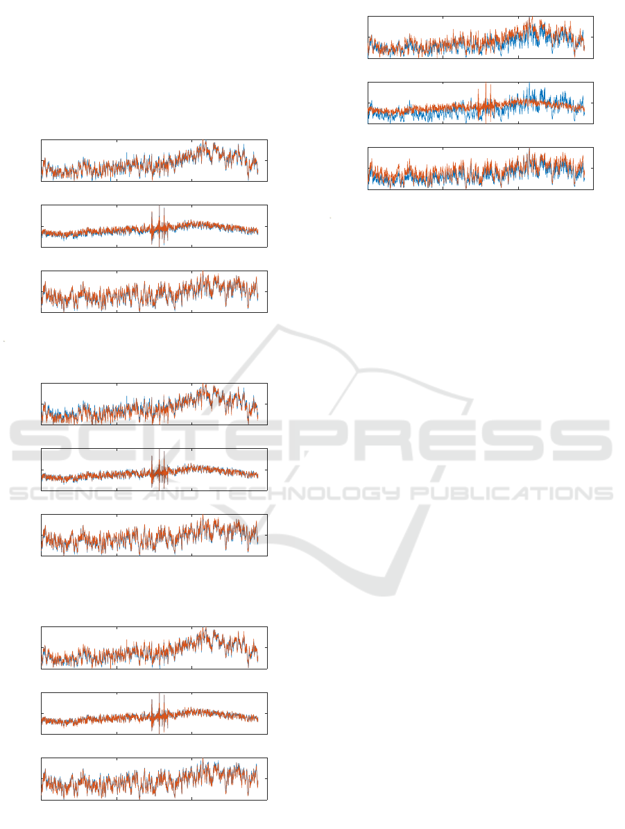
identification approaches are presented by displaying
the plots of the temperatures generated through the
Simulink model and the temperatures predicted by the
identified model. Under the approach of estimating
the low rank approximation of the parameter tensor in
figures 5 and 6, two cases are considered. Case one
with r = 1 and second case with r = 10.
0 500 1000 1500
Sample Number
0
0.5
1
Normalized t
1
0 500 1000 1500
Sample Number
0
0.5
1
Normalized t
2
0 500 1000 1500
Sample Number
0
0.5
1
Normalized t
3
Figure 3: Grey box: measured (red) vs estimated (blue).
0 500 1000 1500
Sample Number
0
0.5
1
Normalized t
1
0 500 1000 1500
Sample Number
0
0.5
1
Normalized t
2
0 500 1000 1500
Sample Number
0
0.5
1
Normalized t
3
Figure 4: Black box: measured (red) vs estimated (blue).
0 500 1000 1500
Sample Number
0
0.5
1
Normalized State t
1
0 500 1000 1500
Sample Number
0
0.5
1
Normalized State t
2
0 500 1000 1500
Sample Number
0
0.5
1
Normalized State t
3
Figure 5: Black box rank 10 approximation: measured (red)
vs estimated (blue).
0 500 1000 1500
Sample Number
0
0.5
1
Normalized State t
1
0 500 1000 1500
Sample Number
0
0.5
1
Normalized State t
2
0 500 1000 1500
Sample Number
0
0.5
1
Normalized State t
3
Figure 6: Black box rank 1 approximation: measured (red)
vs estimated (blue).
From the figures 3, 4 and 5, it is clear that the tem-
peratures predicted by the identified models and the
temperatures generated through the Simulink model
are in agreement. A similar accuracy in identifica-
tion is not seen in figure 6. This means that the pa-
rameter tensor of the model to be identified has a CP
rank substantially higher than 1. Therefore, a rank 1
CP parameter tensor does not adequately represent the
model. The figures 5 and 6 also illustrate the trade off
that is storage effort (r = 1 has 22 elements and r = 10
has 220 elements) and accuracy of the decomposed
tensor with respect to the original parameter tensor.
6 CONCLUSIONS
The paper presents the system identification of an
MTI state space model of a given order using both the
grey and black box identification methods. Within the
black box method, two different approaches are pre-
sented. The first approach focuses on solving an in-
verse problem. The result of this approach is a full
parameter matrix of the state space model. The sec-
ond approach focuses on finding a low rank approxi-
mation of the parameter tensor directly from the mea-
surements.
A numerical example of identification of MTI
state space model for a heating system of an industrial
building was also presented where, state space models
of order three were identified for the corresponding
input-output data sets. Real measurement data was
not available, therefore, virtual data was generated
by simulating a known model of the heating system
in MATLAB Simulink. The data was collected for a
whole day, with signals as close to reality as possible.
The future work should be towards making the es-
timation process more robust to noises. Furthermore,
identification could be carried out for larger systems
with real measurement data.
Approaches to Parameter Identification for Hybrid Multilinear Time Invariant Systems
261

ACKNOWLEDGEMENTS
This work was partly supported by the project
SIOSTA of the Federal Ministry of Education and Re-
search, Germany (Grant-No.: 01LY1812B).
REFERENCES
Lichtenberg, G. (2011). Hybrid tensor systems. Habilita-
tion, Hamburg University of Technology, 152.
Chavan, S. L., & Talange, D. B. (2018). System identifi-
cation black box approach for modeling performance
of PEM fuel cell. Journal of Energy Storage, 18, 327-
332.
Tayamon, S., Zambrano, D., Wigren, T., & Carlsson, B.
(2011). Nonlinear black box identification of a se-
lective catalytic reduction system. IFAC Proceedings
Volumes, 44(1), 11845-11850..
Royer, S., Thil, S., Talbert, T., & Polit, M. (2014). Black-
box modeling of buildings thermal behavior using sys-
tem identification. IFAC Proceedings Volumes, 47(3),
10850-10855.
Bacher, P., & Madsen, H. (2011). Identifying suitable mod-
els for the heat dynamics of buildings. Energy and
Buildings, 43(7), 1511-1522.
Batselier, K., Ko, C. Y., Phan, A. H., Cichocki, A.,
& Wong, N. (2018). Multilinear state space system
identification with matrix product operators. IFAC-
PapersOnLine, 51(15), 640-645.
Kruppa, K. (2017). Comparison of tensor decomposition
methods for simulation of multilinear time-invariant
systems with the MTI toolbox. IFAC-PapersOnLine,
50(1), 5610-5615.
Kolda, T. G., & Bader, B. W. (2009). Tensor decompositions
and applications. SIAM review, 51(3), 455-500.
Cichocki, A., Zdunek, R., Phan, A. H., & Amari, S. I.
(2009). Nonnegative matrix and tensor factorizations:
applications to exploratory multi-way data analysis
and blind source separation. John Wiley & Sons.
Pangalos, G., Eichler, A., & Lichtenberg, G. (2015). Hybrid
multilinear modeling and applications. In Simulation
and Modeling Methodologies, Technologies and Ap-
plications (pp. 71-85). Springer, Cham.
Pangalos, G. (2016). Model-based controller design meth-
ods for heating systems. Technische Universit
¨
at Ham-
burg.
Kruppa, K., & Lichtenberg, G. (2017). Decentralized State
Feedback Design for Multilinear Time-Invariant Sys-
tems. IFAC-PapersOnLine, 50(1), 5616-5621.
Ljung, L. (1999). System identification: theory for the user.
PTR Prentice Hall, Upper Saddle River, NJ, 1-14.
Palensky, P. (2003). The JEVis system-An advanced
database for energy-related services. na.
SIMULTECH 2020 - 10th International Conference on Simulation and Modeling Methodologies, Technologies and Applications
262
