Scalable Electric-motor-in-the-Loop Testing for Vehicle Powertrains

Thomas D’hondt

1 a

, Yves Mollet

1,2 b

, Arthur Jacques Joos

, Leonardo Cecconi

Mathieu Sarrazin

and Johan Gyselinck

2 c

Test Division, Siemens Industry Software NV, Researchpark 1237, Interleuvenlaan 68, B-3001 Leuven, Belgium

BEAMS Department, Universit

e Libre de Bruxelles, Avenue Franklin Roosevelt 50, CP165/52, B-1050 Bruxelles, Belgium

Keywords:

Electric Vehicles, e-Powertrain, Model-Based System Testing, Scaling, Real-time Control, X-in-the-Loop.

Abstract:

Model-Based System Testing (MBST) combines physical testing and simulation models to enable the valida-

tion of complex systems early-on in their design cycle. Therefore, it shows great potential for the validation

of increasingly complex Electric Vehicle (EV) powertrains. In this work, the MBST methodology is applied

to a downscaled powertrain, including a Permanent-Magnet Synchronous Machine (PMSM) and a 3-phase

switch-mode inverter. This System-under-Test (SuT) is integrated into an X-in-the-Loop (XiL) test bench,

where real-time simulation models of the rest of the vehicle are used to impose realistic boundary conditions

to the SuT. These include the emulation of the vehicle inertia, its friction losses and the regenerative braking

controller. Both hardware and software architectures required to achieve this setup are presented. Subse-

quently, a methodology used for computing scaling factors that match the power levels of the full vehicle to

the miniature test bench is proposed. Finally, the combined physical-virtual system is evaluated on a driving

cycle to validate its behaviour. The usage of a downscaled SuT constitutes the ﬁrst step towards full-scale

E-powertrain-in-the-loop testing, as well as a valuable multi-purpose didactical XiL setup.

1 INTRODUCTION

In Model-Based System Testing (MBST), simulation

models and physical testing are combined to inves-

tigate, improve or validate complex multi-physical

or mechatronic systems (Siemens Digital Industries

Software, 2019). In this framework, X-in-the-Loop

(XiL) testing is more speciﬁcally used to test one or

more physical components, while simulating their en-

vironment, such that the physical presence of the sur-

rounding hardware is not required to create realistic

working conditions (Van der Auweraer et al., 2017).

As a consequence, XiL-based prototyping can be per-

formed at early development stages and requires lim-

ited hardware compared to its physical counterpart,

permitting a shorter time-to-market and lower devel-

opment costs (Fathy et al., 2006).

This technique is particularly interesting for re-

search and development in Electric Vehicles (EVs),

especially focusing on drivetrain (Popp et al., 2015;

Petersheim and Brennan, 2009; Yang et al., 2015) and

https://orcid.org/0000-0003-2554-332X

https://orcid.org/0000-0001-6170-0148

https://orcid.org/0000-0003-2259-8560

consumption (Ciceo et al., 2016; Williamson et al.,

2006) to address their present shortages in efﬁciency,

autonomy and acoustic comfort, in the challenging

context of more and more restrictive ecological and

safety regulations (Fiori et al., 2016; Yang et al.,

2014). In this domain, XiL testing also allows for

high repeatability compared to real driving and may

avoid increased computation time or resources in case

of full-vehicle simulation (Fathy et al., 2006). This is

of paramount interest as more complex powertrains

and increasing amounts of electrical accessories can

result in integration issues if combined late in the de-

sign process. Therefore, the application of the MBST

methodology on EVs is currently being studied in the

OBELICS (Optimization of scalaBle rEaltime mod-

eLs and functIonal testing for e-drive ConceptS) re-

search project (Obelics consortium, 2019).

A surrogate System-under-Test (SuT) can be used

to reduce prototyping costs when the original hard-

ware is not required for the investigations of inter-

est (Petersheim and Brennan, 2009). Adequate scal-

ing factors allow then to match the characteristics of

the SuT to the model. This principle is used in the

present paper to signiﬁcantly downscale the surrogate

SuT compared to similar setups (Popp et al., 2015;

594

D’hondt, T., Mollet, Y., Joos, A., Cecconi, L., Sarrazin, M. and Gyselinck, J.

Scalable Electric-motor-in-the-Loop Testing for Vehicle Powertrains.

DOI: 10.5220/0009887405940603

In Proceedings of the 17th International Conference on Informatics in Control, Automation and Robotics (ICINCO 2020), pages 594-603

ISBN: 978-989-758-442-8

Real-time simulation model

Test bench

Traction

inverter

Load

inverter

LoadTraction

Downscale

Upscale

Vehicle

dynamics

Vehicle

Control Unit

Driver

Reference

proﬁle

˙x

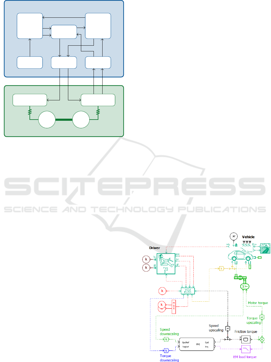
Figure 1: Overview of the test bench layout and of the con-

nected simulation models. The variables with tilde corre-

spond to the reduced-scale test bench.

Petersheim and Brennan, 2009; Ciceo et al., 2016).

This reduction in size does not only reduce material

costs, but also has a two-fold objective: propose a safe

validation step between pure simulations and full-size

test environments, as well as a valuable and trans-

portable didactic / demonstration setup. Indeed, it can

be used to evaluate control strategies on a state-of-

the-art test bench controller and inverter, while stay-

ing in a low-risk environment. The bench comprises

two low-power Permanent-Magnet Synchronous Ma-

chines and their respective inverters. One Permanent-

Magnet Synchronous Machine (PMSM) and its in-

verter constitute the surrogate SuT, receiving a torque

reference from the throttle, whereas the other emu-

late the behaviour of a real car via a speed refer-

ence. It is obtained by a real-time model of the rest of

the car combined with adequate scaling factors (Fig-

ure 1). Furthermore, although this article considers an

EV context, the test bench may be used for XiL tests

where other environments are simulated.

This paper ﬁrst describes in detail the real-time

simulation models which are used to provide realis-

tic boundary conditions to the SuT and how they are

integrated into the overall controller of the test bench.

The physical layout of the test bench is then investi-

gated and scaling factors are computed to match the

power level in the simulation model to that of the

physical components. Finally, the ﬁrst experimental

results and conclusions are presented.

2 REAL-TIME SIMULATION

MODELS

The real-time simulation model used to provide real-

istic boundary conditions to the SuT (Figure 1) con-

sists of three major subsystems: (i) the driver, (ii) the

Vehicle Control Unit (VCU) and (iii) the dynamics of

the rest of the vehicle. This last part of the model

includes the behaviour of the car body, gearbox and

brakes. All of them are implemented considering a

BMW i3 as a full-scale reference EV (BMW, 2017).

Their overall implementation in the Simcenter

Amesim software (Figure 2), as well as the corre-

sponding parameters, will be further explained in this

section. The computation of the scaling factors used

to match the characteristics of the reference vehicle

to the physical limitations of the test bench will be

investigated in Section 5.

2.1 Driver

The aim of the driver is to compute the adequate throt-

tle and brake commands to be applied to the vehi-

cle, u

and u

respectively. This closed-loop con-

troller therefore takes the measured longitudinal ve-

hicle speed ˙x and tries to make it track a pre-deﬁned

velocity proﬁle ˙x

(Figure 1). Those proﬁles can,

for instance, be the New European Driving Cycle

(NEDC) or World harmonised Light vehicles Test Cy-

cle (WLTC) for assessing the energy consumption of

the vehicle. In the remainder of the paper, the super-

scripts m and r will refer to measured and reference

Figure 2: Vehicle simulation model generated in Simcenter

Amesim.

Scalable Electric-motor-in-the-Loop Testing for Vehicle Powertrains

595

˙x

−

˙x

Anticipative

PI throttle

PI brake

−1

Figure 3: Driver controller layout.

quantities respectively. Similarly, the subscripts t and

b correspond to the throttle and brake actions. Finally,

tilde variables are referred to the reduced-power test

bench, whereas regular variables correspond to the

full-scale EV.

Two independent Proportional Integral (PI) con-

trollers with an additional anticipative action are used

to compute the vehicle inputs (Figure 3). The antici-

pative action is calculated using an approximated ref-

erence acceleration:

˙x

(t + ∆T )− ˙x

(t)

∆T

, (1)

where ∆T is the anticipative time constant. It is then

multiplied by throttle- and brake-speciﬁc gains and

summed to the outputs of the regular PI controllers.

Finally, both the throttle and braking action are satu-

rated in the [0,1] interval.

2.2 Vehicle Control Unit

The VCU converts the computed throttle and brake

commands into a reference torque for the E-motor τ

and for the mechanical brakes τ

, taking regenerative

braking into account (Figure 1). Therefore, a user-

requested torque τ

is ﬁrst computed by transforming

the normalised user inputs into a torque value:

= u

max

+ u



min

−

max



, (2)

where τ

max

> 0 and τ

min

≤ 0 are the maximum E-

motor torques in motoring and braking operation. The

maximum mechanical braking torque τ

max

> 0 of the

vehicle is referred to the shaft of the E-motor by di-

viding it by the gearbox ratio r. The user-requested

torque τ

is then split according to a ﬁxed repartition

strategy (Figure 4). The blue and green areas rep-

resent the contribution of τ

and τ

to the total ve-

hicle torque referred to the E-motor shaft. During

the braking operation, the ﬁxed ratio is held until τ

reaches the braking torque limit of the E-motor τ

min

Although not further studied in this paper, the regen-

erative action can also be inhibited at too low or too

high speeds and depending on battery state-of-charge.

2.3 Vehicle Dynamics

The vehicle body is simulated as a point-mass moving

in the longitudinal dimension x. The equivalent mass

of the vehicle includes both the vehicle mass M and

its wheel inertia J



M + 4



¨x =

rτ

−τ

−F

, (3)

with R

, τ

and τ

the wheel radius, the measured

and upscaled E-motor torque and the braking torque.

Both torques are transformed into longitudinal forces

considering the ﬁxed and unitless reducer gear ratio r

and the wheel radius R

. Finally, the resistive force

exerted by the environment on the car F

comprises

both aerodynamic drag and rolling resistance:

air

˙x

+ Mg(a + b ˙x), (4)

with ρ

air

the air density, C

the air penetration coefﬁ-

cient and S the vehicle active area. No external wind

is currently considered in the aerodynamic drag term.

The rolling resistance is supposed to be proportional

to the vehicle mass M and the gravity g with a con-

stant term a and a term proportional to the vehicle

speed b ˙x. It should be noted that no slope, nor stic-

tion effects are considered in the present paper.

A friction torque compensation mechanism is in-

cluded in the simulation model due to the non-

negligible friction in the test setup compared to the

nominal torque of the machines. Indeed, the elec-

tromagnetic torque

estimated by the load inverter

based on current measurements differs from the elec-

tromagnetic torque

from the SuT motor expected

by the vehicle simulation model. The difference be-

tween both corresponds to the friction of the loading

max

min

−

max

min

−

max

min

Electrical motoring and

braking torque τ

Mechanical braking

torque at motor shaft τ

Figure 4: Split between regenerative and mechanical

torques during braking manoeuvres.

ICINCO 2020 - 17th International Conference on Informatics in Control, Automation and Robotics

596

−4 −2 0 2 4

−40

−20

Rotation speed [krpm]

Friction torque [mNm]

Measured points

Interpolated data

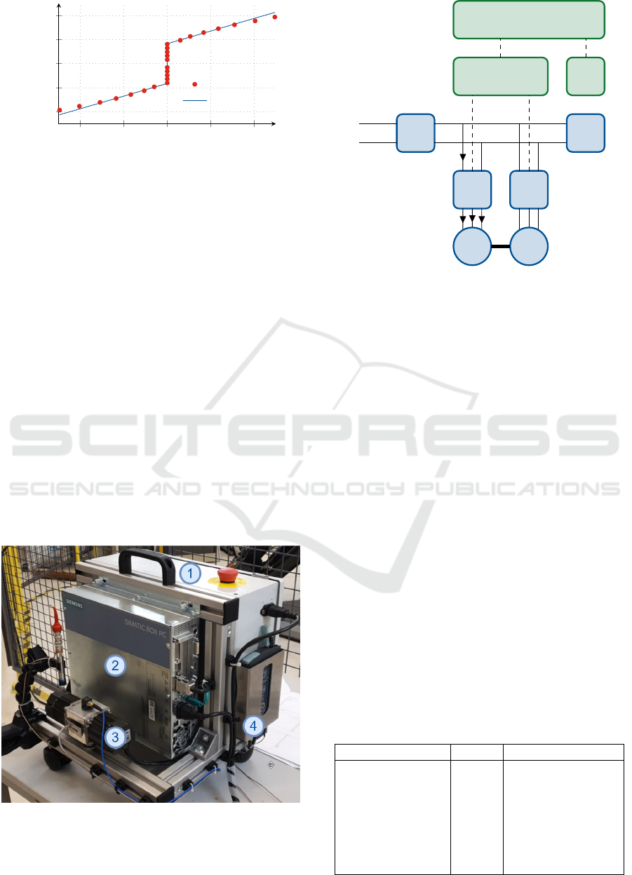
Figure 5: Test bench friction

as a function of rotational

speed

machine

, which is identiﬁed during pre-

liminary tests at constant speed and approximated us-

ing a ﬁrst-order relation:

(

) = sign(

)



f ,0

+ K



, (5)

where τ

f ,0

and K

are the static and dynamic friciton

coefﬁcients. The measured and interpolated data used

in the simulation model are represented in Figure 5.

3 CONSTRUCTION OF THE XiL

TEST BENCH

The downscaled XiL test setup created for this work

consists of three main subsystems: (i) the power cab-

inet, (ii) the real-time computing unit and (iii) the E-

motor testbed. All three are visible in Figure 6.

The power cabinet and the testbed contain two

motor and inverter pairs: the powertrain-under-test

Figure 6: The power supply and inverters are located inside

the electrical power cabinet (1). The real-time controller (2)

is ﬁxed on a frame, which also supports the electric motors

using a small vibration absorber (3). A DAQ is mounted on

the side of the setup (4).

PSU

230 V

Traction

inverter

Load

inverter

Braking

resistor

Traction Load

Real-time controller

CAN EC

DAQ

Operator computer

ETH ETH

Figure 7: Electrical scheme of the test setup.

and its load (Figure 7). Both traction and load motors

use the same low-power PMSM, whose speciﬁcations

are provided in Tables 1 and 2. Their rotor shafts are

connected through a spider coupling, while their sta-

tors are rigidly mounted and aligned with a metallic

bracket.

The traction motor is controlled by a Texas In-

struments (TI) inverter development kit, whose torque

control algorithms can be freely tuned by the test

engineer (Texas Instruments, 2017). Its controller

chip is similar to the ones used in commercial road

car powertrain applications; only the power levels

are reduced. The load motor is controlled by a

maxon EPOS 3 industrial inverter, which operates in

speed-controlled mode. Finally, a 37.3 V DC-bus is

provided by a regular industrial Power Supply Unit

(PSU), which is protected from over-voltage during

sudden braking manoeuvres by a braking resistor and

a chopper. Both inverters share their DC-bus to enable

the recirculation of the generated power.

The test bench is controlled from a real-time com-

puting unit whose objectives are twofold: (i) execute

the above detailed real-time simulation model of the

vehicle and of the driver and (ii) handle the commu-

nication between the simulation model and the phys-

Table 1: Speciﬁcations of the PMSM used on the testbed.

Parameter Symb. Value

Pole pairs p 4

Voltage constant K

4.75 V

ph−ph

/krpm

Torque constant K

0.04533 N m/A

Stator resistance R

0.36 Ω (25

◦

d-axis inductance L

0.201 mH

q-axis inductance L

0.201 mH

Rotor inertia J

7 kg mm

Scalable Electric-motor-in-the-Loop Testing for Vehicle Powertrains

597

Co-simulation master

FMI

slave

CAN

slave

Data

logger

Conﬁguration

Data

ﬁle

Figure 8: Structure of the real-time controller. Blue, green

and purple blocks correspond to hard real-time processes,

non-real-time processes and output ﬁles respectively.

ical components on the testbed (Figure 7). As in a

real automotive use case, the torque

requested by

the VCU and the inverter state transitions are sent to

the TI inverter over Controller Area Network (CAN).

The maxon load inverter communicates the measured

load torque

and speed

to the controller and

receives its new reference speed

using the indus-

trial ﬁeld bus EtherCAT (EC) (EtherCAT Technology

group, 2019). Finally, a Simcenter SCADAS Data-

Acquisition System (DAQ) is included in the setup to

measure the speed

and two phase currents

and

(the last current

being computed as

= −

−

) of

the surrogate PMSM, as well as the current

ﬂow-

ing from the DC-bus to the traction inverter during

the execution of the tests. Both this DAQ and the

real-time computing unit are conﬁgured via Ethernet

(ETH) from an operator computer.

4 REAL-TIME CONTROL

STRUCTURE

The real-time computing unit is responsible for the

execution of simulation models and the interfacing

between them and with the physical components on

the test bench. For this purpose, a real-time co-

simulation architecture is set up within the unit, which

is functionally divided into a master and several slaves

(Figure 8).

The co-simulation master orchestrates the execu-

tion and data exchange of the different co-simulation

slaves. The master execution is scheduled by a low

jitter real-time timer, ﬁring every master timestep t

At the beginning of each timestep, the master triggers

the execution of the slaves and waits for them to return

outputs. Co-simulation correction algorithms are then

run on the resulting outputs and the corrected values

are propagated to the respective slave inputs. Finally,

the master waits for the end of the current timestep

unless an overrun occurred (Figure 9).

In the present application, a co-simulation slave

exposing a Functional Mock-up Interface (FMI) is

used to execute the Amesim model (Blochwitz et al.,

2012). Apart from the execution of the simulation

models, co-simulation slaves are also responsible for

speciﬁc functionalities of the controller, such as the

handling of physical I/O. Indeed, both CAN and

EtherCAT slaves are used to communicate with the

traction and load inverter respectively.

In general, the computation rate of the master can

differ from the one of the slaves. Indeed, the co-

simulation slaves can run their models once or more

per master timestep t

to ensure a speciﬁc virtual rate

for the numerical integration, where n

is the num-

ber of micro-steps of the ith slave. Subsequently, their

results are returned to the master for synchronisation

and exchange (Gomes et al., 2017). Due to the mas-

ter pacing at a lower rate, the slaves see their inputs

updated only once every n

steps. This could intro-

duce artefacts in the co-simulation and generate non-

physical frequency content in the signals. To miti-

gate this effect, the co-simulation master implements

numerical techniques aiming to reconstruct the be-

haviour of the input signals locally to the slave during

isolation. An example of such method is provided in

(Stettinger et al., 2014).

Each of the previously mentioned slaves, as well

as the master, are executed in separate processes and

on different CPU cores of the real-time computing

unit to minimise computational time jitter. In fact, the

most important requirement for a real-time system is

time determinism over the carried-out operations. For

this reason, the real-time unit is based on a real-time

patched (Real-Time Linux Wiki, 2016) Linux kernel

that runs the operating system as a fully preemptive

process, hence increasing scheduling and computa-

tional time determinism.

CAN slave

EC slave

FMI slave

Master

Figure 9: Timing diagram of the real-time controller.

ICINCO 2020 - 17th International Conference on Informatics in Control, Automation and Robotics

598

5 INTRODUCTION OF SCALING

FACTORS

Scaling factors are used to match the full-scale real-

time model to the reduced-scale test bench. These co-

efﬁcients are calculated following the approach used

in (Petersheim and Brennan, 2009). The relevant pa-

rameters for motor scaling are ﬁrst identiﬁed, based

on the torque-speed curve and the limitations of the

motor: the maximum motor torque τ

max

, the maxi-

mum power P

max

, the maximum speed ω

max

, the ro-

tational speed ω and the motor torque τ. The values

of τ

max

, ω

max

and P

max

are listed for the EV motor

and for the surrogate PMSM, both with and with-

out considering friction, in Table 2. Three dimen-

sionless variables are then deduced based on the the-

ory of Applied Dimensional Analysis and Modelling

(Szirtes and R

ozsa, 2007): π

max

, π

max

and

max

. The detailed calculation of the dimen-

sionless variables can be found in (Joos, 2019).

By using reduced variables π

and π

, the torque-

versus-speed curves of the EV motor and small

PMSMs used on the bench can be plotted along nor-

malised axes, as shown in Figure 10. However, the

shapes of the curves do not match: the curve of the

EV motor consists of a hyperbolic curve in the ﬂux

weakening zone, i.e. where the maximum power is

the main limitation of the machine. On the contrary,

the ideal torque-versus-speed curve of the PMSM of

the test bench presents a wide linear part, as the max-

imum continuous power is only reached close to the

maximum speed. A better match of both curves could

be obtained by performing ﬂux weakening on the test

bench motor, but falls out of the scope of this paper,

as safety margins must be deﬁned to avoid demag-

netization of the permanent magnets. Furthermore,

considering the non-negligible friction torque on that

machine, its corrected curve shows a maximum shaft

torque decreasing with speed as the friction torque in-

creases.

Considering the curves in Figure 10, a small area

(at low speed and high torque) can be observed where

the curve of the surrogate PMSM with friction is lo-

cated below the one of the EV motor. Therefore, those

operating points of the EV motor correspond to an

overload of the test bench PMSM. However, when

plotting the scaled working points corresponding to

the NEDC and WLTC, no point falls in that region

and an important margin can even be seen. There-

fore, these scaling factors ensure a safe operation of

the bench for testing such driving cycles.

By equalling the dimensionless variables for both

machines, the scaling factors for torque and speed can

be easily computed as the ratios between maximum

torques

max

and speeds

max

of both machines. For

sake of simplicity, the scaling factors are chosen for

the XiL tests without considering friction in Table 2,

i.e.

max

= 1.03 ×10

−3

and

max

= 0.517.

6 XiL TEST RESULTS

Closed-loop XiL tests are performed to validate this

scalable testing approach. Detailed results on the ﬁrst

part of the NEDC (0 s to 30 s) are ﬁrst discussed be-

fore showing the overall bench performance on the

whole cycle. The evolution of speed, currents and

torque on the surrogate PMSM are displayed in Fig-

ures 11, 12 and 13 respectively.

In Figure 11 the shaft speed

of the surrogate

SuT measured with the Simcenter SCADAS is com-

pared to the theoretical proﬁle of the NEDC converted

in terms of speed of the EV motor.

Figure 11 shows that the speed proﬁle of the

NEDC is globally well followed for the small-scale

SuT, similarly to the results presented in (Petersheim

and Brennan, 2009; Ciceo et al., 2016) for normal-

scale benches. Some delays can, however, be reduced

through an improved tuning of the driver parameters.

The more important delay in the decelerating slope

can be linked to the use of different controller pa-

rameters for acceleration and braking, as presented in

Figure 3. When the reference speed starts decreas-

ing, there is a small delay between the time the accel-

eration controller stops acting to counter the friction

(i.e. the driver releases the throttle) and the time the

braking controller starts acting (i.e. the driver starts

pressing on the braking pedal). The absence of anti-

wind-up loops on these controllers is the most proba-

0 0.1 0.2 0.3 0.4 0.5 0.6 0.7 0.8 0.9 1

-0.2

0.2

0.4

0.6

0.8

EV motor

PMSM motor (w/o friction)

PMSM motor (w/ friction)

NEDC

WLTC

PMSM overload

Figure 10: Dimensionless plot of the torque-versus-speed

curves of the real and surrogate SuTs, with operating point

for two different driving cycles.

Scalable Electric-motor-in-the-Loop Testing for Vehicle Powertrains

599

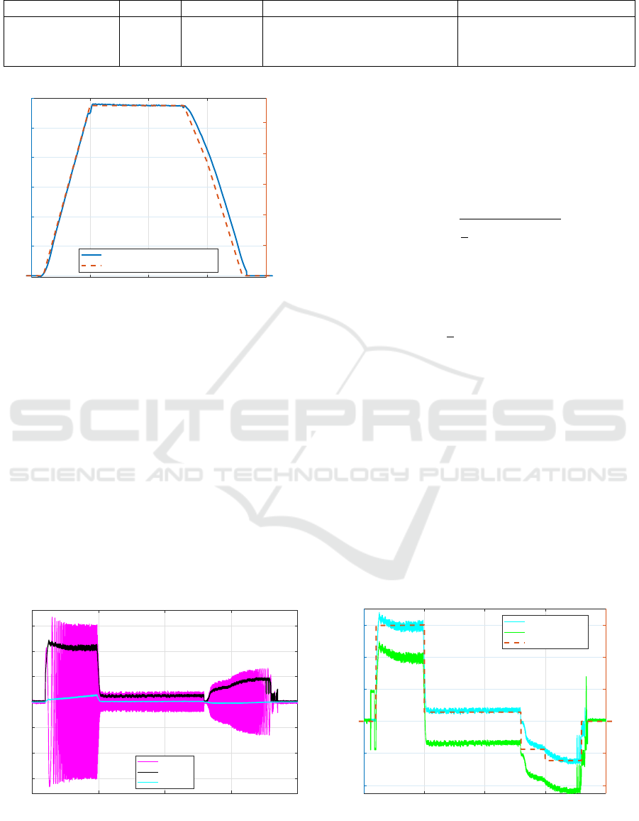
Table 2: Maximum ratings of the EV and surrogate SuT motors.

Parameter Symbol Value (EV) Value (PMSM without friction) Value (PMSM with friction)

Maximum speed ω

max

11.6 krpm 6 krpm 6 krpm

Maximum torque τ

max

270 N m 279 mN m 263 mN m

Maximum power P

max

75 kW 171.7 W 151.2 W

10 15 20 25 30

Time [s]

100

200

300

400

500

600

Test bench speed [rpm]

200

400

600

800

1000

EV motor speed [rpm]

Measured scaled speed

Linear speed from NEDC profile

Figure 11: Speed proﬁle

of the surrogate SuT and the

ﬁrst part of the urban cycle of the NEDC.

ble explanation.

Looking in greater detail at Figure 11, a small

bump can be observed prior to the plateau speed cor-

responding to 15 s in the NEDC. It is probably due to

the anticipative action of the acceleration controller,

monitoring the difference between present and fu-

ture (0.1 s later) speed set-points. Furthermore, just

before the begin of the rising slope at 11 s, a very-

low-amplitude negative speed is measured, probably

due to some backwards movement of the rotor at the

bench start-up. The traction inverter does not seem to

be responsible for this, as the phase currents in Fig-

ure 12 only show noise before 11 s.

Figure 12 presents the measured currents

, and

10 15 20 25 30

Time [s]

-1.5

-1

-0.5

0.5

1.5

Current [A]

Phase a

AC RMS

Figure 12: DC-bus, phase and estimated RMS currents in

the surrogate SuT during the ﬁrst part of the urban cycle of

the NEDC.

on the SuT. These signals are displayed after hav-

ing been ﬁltered with a zero-phase second-order But-

terworth ﬁlter with a 2 kHz cut-off frequency. This

ﬁltering is required to match the hypothesis of sinu-

soidal and balanced phase currents needed to estimate

the value of the AC RMS current (also displayed in

Figure 12) with the following formula:

rms





, (6)

where the e superscript reﬂects the estimated nature of

this quantity. It is then used together with the torque

constant of the machine K

to estimate the torque of

the surrogate motor

= K

√

rms

·sign



dc, f iltered



, (7)

where

dc, f iltered

represents

after applying a

second-order Butterworth ﬁlter with a 5.12 Hz cut-

off frequency to prevent noise from affecting the esti-

mated torque direction.

is an estimate of

The electromagnetic torque

of the traction

PMSM of the bench, estimated from (7), is compared

in Figure 13 with the theoretical torque proﬁle to be

applied to the EV motor to follow the NEDC (con-

sidering a constant 57 % ratio of the braking torque

is supplied via the EV motor). An estimate of the

loading-machine torque

using the measurements

acquired with the Simcenter SCADAS is also dis-

played in the ﬁgure. This value is computed from

using (5).

10 15 20 25 30

Time [s]

-40

-20

Electromagnetic torque [mNm]

-40

-20

EV motor torque [Nm]

SUT machine

Loading machine

EV motor

Figure 13: Torques of the surrogate SuT

and loading ma-

chine

(left scale), as well as the corresponding torque for

the real vehicle (right scale).

ICINCO 2020 - 17th International Conference on Informatics in Control, Automation and Robotics

600

10 15 20 25 30

Time [s]

Consumed energy (bench) [J]

Consumed energy (EV) [Wh]

DC bus (PMSM)

PMSM shaft (w/o friction)

DC bus (EV)

EV motor shaft (w/o friction)

Figure 14: Consumed energy by the surrogate SuT and the

corresponding energy requirement from the EV.

The resulting torque proﬁle is globally well followed

with the expected scaling factor. However, some de-

lay is observed due to the driver’s dynamic, as already

shown for the speed proﬁle in Figure 11. The evo-

lution of

shows the important part of the friction,

which is compensated for by feed-forwarding the es-

timated friction torque

in the real-time simulation

model.

Some torque oscillations can be noticed at the be-

ginning and the end of the test. This corresponds to

moments where the motors start or stop their rotation.

The ones of

before the acceleration ramp are prob-

ably nonphysical and linked to the small backwards

movement of the rotor and the way this torque is es-

timated. However, the later oscillations in the SuT

and loading machine torques could have a three-fold

origin. Firstly, the sensorless torque control of the

TI drive, which uses a speed estimator instead of a

sensor, tends to work badly at lower speeds. Indeed,

the estimated direction of rotation can be inaccurate

when its speed is around 0 rpm. Secondly, the load-

ing machine is controlled in block commutation by

the maxon drive, which leads to a jerky torque gen-

eration at lower speeds. Finally, the friction torque

compensation provided in (5) also shows a disconti-

0 2000 4000 6000 8000 10000

Speed [rpm]

100

150

200

250

Torque [Nm]

0.25

0.5

0.6

0.7

0.75

0.8

0.825

0.85

0.875

0.9

0.91

0.92

0.93

Figure 15: Estimated efﬁciency map of the EV motor.

0 200 400 600 800 1000 1200

Time [s]

500

1000

1500

2000

2500

3000

3500

4000

4500

Test bench speed [rpm]

Scaled actual speed

Scaled reference speed

Figure 16: Actual

and reference speeds of the surrogate

SuT for the full NEDC.

nuity around 0 rpm, which could result in jumps in τ

that propagate across the real-time simulation model.

Figure 14 shows the amount of energy absorbed

by the traction inverter and delivered to the shaft of

the surrogate PMSM excluding friction. For compar-

ison, their theoretical counterparts computed directly

from the NEDC speed proﬁle for the EV motor are

displayed as well, considering the assumptions made

in (Joos, 2019) regarding the EV motor and converter

efﬁciencies. While a constant 95 % converter efﬁ-

ciency is assumed, the efﬁciency map of the EV mo-

tor is computed by adding a 15 % constant offset to

the one of the surrogate PMSM, leading to the map

displayed in Figure 15.

It appears that the consumed energies at the shaft

match relatively well, even if an increased difference

can be seen during the decelerating ramp, due to the

delay between the measured speed and the theoretical

one. However, the energies taken from the DC-bus or

battery differ, due to the different motor efﬁciencies.

The scaled reference and actual speeds of the load-

ing PMSM extracted from the Amesim model over

the whole NEDC are shown in Figure 16. They show

0 200 400 600 800 1000 1200

Time [s]

100

120

140

160

180

Energy consumption [Wh/km]

Figure 17: Estimated energy consumed at battery terminals

for the real vehicle over the NEDC based on torque and

speed measurements on the surrogate SuT.

Scalable Electric-motor-in-the-Loop Testing for Vehicle Powertrains

601

a good tracking of the reference speed by the maxon

drive, as the NEDC proﬁle is easily recognisable.

Finally, the estimated consumed energy per kilo-

meter at the EV battery terminals is displayed in Fig-

ure 17 (considering the same assumptions as for Fig-

ure 14). The ﬁnal value of this plot (168 Wh/km) is

17.5 % higher than the claimed consumption of the

modelled EV, i.e. 143 Wh/km (BMW, 2017). Such

an overestimation can be expected, since the raw es-

timation of the motor and converter efﬁciencies are

very probably underestimations.

7 CONCLUSIONS

In this work, the MBST methodology has been suc-

cessfully applied to a downscaled XiL test setup used

for the validation of EV powertrains, thanks to ade-

quate scaling factors. Validation has been performed

on the NEDC. The results also show the inﬂuence of

the control strategy on the tracking of the speed pro-

ﬁle and suggests a possible future use of the small-

scale bench for control optimisation.

In future work, the authors will build on this work

to increase the power level of the SuT and show

the scalability of the proposed framework to real EV

components. Additionally, the didactic side of this

downscaled setup will be further exploited by further

extending its instrumentation. The present PMSM

used in SuT will also be exchanged with an induc-

tion motor of similar power to enable testing this type

of traction motors.

ACKNOWLEDGEMENTS

This project was partially funded by the European

Union’s Horizon 2020 research and innovation pro-

gram under grant agreement No 769506.

The content of this publication does not reﬂect the of-

ﬁcial opinion of the European Union. Responsibility

for the information and views expressed therein lies

entirely with the authors.

REFERENCES

Blochwitz, T., Otter, M.,

Akesson, J., Arnold, M., Clauß,

C., Elmqvist, H., Friedrich, M., Junghanns, A.,

Mauss, J., Neumerkel, D., Olsson, H., and Viel,

A. (2012). Functional mockup interface 2.0: The

standard for tool independent exchange of simulation

models. In Proceedings of the 9th International Mod-

elica Conference.

BMW (2017). Speciﬁcations. the new bmw i3. In BMW

media information, pages 1–8.

Ciceo, S., Mollet, Y., Sarrazin, M., Van der Auweraer, H.,

and Martis, C. (2016). Model-based design and test-

ing for electric vehicle energy consumption analysis.

Electrotehnic

a, Electronic

a, Automatic

a, 64:46–51.

EtherCAT Technology group (2019). EtherCAT. www.

ethercat.org. Accessed: 2019-08-05.

Fathy, H. K., Filipi, Z. S., Hagena, J., and Stein, J. (2006).

Review of hardware-in-the-loop simulation and its

prospects in the automotive area. Proceedings of SPIE

- The International Society for Optical Engineering,

6228.

Fiori, C., Ahn, K., and Rakha, H. A. (2016). Power-

based electric vehicle energy consumption model:

Model development and validation. Applied Energy,

168:257–268.

Gomes, C., Thule, C., Larsen, P. G., and Vangheluwe, H.

(2017). Co-simulation: State of the art.

Joos, A. J. (2019). Implementation of a small-scale elec-

trical drive system in Hardware-in-the-Loop simula-

tions. Master’s thesis, Brussels Faculty of Engineer-

ing.

Obelics consortium (2019). Homepage - Obelics. obelics.

eu. Accessed: 2019-08-05.

Petersheim, M. D. and Brennan, S. (2009). Scal-

ing of hybrid-electric vehicle powertrain components

for hardware-in-the-loop simulation. Mechatronics,

19:1078–1090.

Popp, A., Sarrazin, M., Van der Auweraer, H., Fodorean,

D., Birte, O., Karoly, B., and Martis, C. (2015). Real-

time co-simulation platform for electromechanical ve-

hicle applications. 2015 9th International Symposium

on Advanced Topics in Electrical Engineering, pages

240–243.

Real-Time Linux Wiki (2016). Real-Time Linux Wiki.

rt.wiki.kernel.org/index.php/Main Page. Accessed:

2020-04-01.

Siemens Digital Industries Software (2019). Model-

based system testing: Efﬁciently combining test

and simulation for model-based development.

https://www.plm.automation.siemens.com/media/

global/en/Model-based%20system%20testing%

20WP tcm27-67978.pdf.

Stettinger, G., Horn, M., Benedikt, M., and Zehetner, J.

(2014). Model-based coupling approach for non-

iterative real-time co-simulation. In 2014 European

Control Conference (ECC), pages 2084–2089.

Szirtes, T. and R

ozsa, P., editors (2007). Applied Di-

mensional Analysis and Modeling, pages 133 – 161.

Butterworth-Heinemann, Burlington, 2nd edition.

Texas Instruments (2017). InstaSPIN-FOC and InstaSPIN-

MOTION User’s Guide. http://www.ti.com/lit/ug/

spruhj1g/spruhj1g.pdf. Accessed: 2019-08-05.

Van der Auweraer, H., Sarrazin, M., and Marques dos San-

tos, F. (2017). Model-based system testing: A new

ICINCO 2020 - 17th International Conference on Informatics in Control, Automation and Robotics

602

drive to integrating test and simulation. In 2017 In-

ternational Conference on Structural Engineering Dy-

namics.

Williamson, S., Lukic, M., and Emadi, A. (2006). Compre-

hensive drive train efﬁciency analysis of hybrid elec-

tric and fuel cell vehicles based on motor-controller

efﬁciency modeling. IEEE Transactions on power

electronics, 21(3):730–740.

Yang, Y.-P., Shih, Y.-C., and Chen, J.-M. (2014). Real-time

driving strategy for a pure electric vehicle with mul-

tiple traction motors by particle swarm optimization.

7th IET International Conference on Power Electron-

ics, Machines and Drives (PEMD 2014).

Yang, Z., Shang, F., Brown, I. P., and Krishnamurthy, M.

(2015). Comparative study of interior permanent mag-

net, induction, and switched reluctance motor drives

for ev and hev applications. IEEE Transactions on

Transportation Electriﬁcation, 1(3):245–254.

ACRONYMS

CAN Controller Area Network.

DAQ Data-Acquisition System.

EC EtherCAT.

ETH Ethernet.

EV Electric Vehicle.

FMI Functional Mock-up Interface.

MBST Model-Based System Testing.

NEDC New European Driving Cycle.

PI Proportional Integral.

PMSM Permanent-Magnet Synchronous Machine.

PSU Power Supply Unit.

SuT System-under-Test.

TI Texas Instruments.

VCU Vehicle Control Unit.

WLTC World harmonised Light vehicles Test Cycle.

XiL X-in-the-Loop.

SYMBOLS

Air penetration coefﬁcient.

Longitudinal resistive force.

Wheel inertia.

M Vehicle mass.

Wheel radius.

S Vehicle active area.

˙x

Reference longitudinal vehicle speed.

˙x Longitudinal vehicle speed.

Measured EV motor rotational speed.

Reference EV motor rotational speed.

air

Air density.

User torque request.

max

Maximum vehicle braking torque.

max

Maximum EV motor torque.

min

Minimum EV motor torque.

Mechanical braking torque.

Measured EV motor torque.

Reference EV motor torque.

Measured SuT rotational speed on the test bench.

Reference SuT rotational speed on the test bench.

Torque at the SuT shaft on the test bench.

Estimated SuT torque on the test bench, based on

Simcenter SCADAS measurements.

Reference SuT torque on the test bench.

Test bench mechanical friction torque.

Estimated load motor torque on the test bench,

based on Simcenter SCADAS measurements.

Measured load motor torque on the test bench.

rms

Estimated RMS current in the phases of the SuT.

Current in the phase a of the SuT.

Current in the phase c of the SuT.

Current in the DC-bus of the SuT.

g Constant of gravity.

r Gearbox ratio.

Brake command.

Throttle command.

x Vehicle longitudinal position.

Scalable Electric-motor-in-the-Loop Testing for Vehicle Powertrains

603