Improved IMU-based Human Activity Recognition using Hierarchical

HMM Dissimilarity

Sara Ashry

1,2

, Walid Gomaa

1,3

, Mubarak G. Abdu-Aguye

and Nahla El-borae

Cyber-Physical Systems Lab (CPS), Computer Science and Engineering Department (CSE),

Egypt-Japan University of Science and Technology (E-JUST), Alexandria, Egypt

Computers and Systems Department, Electronic Research Institute (ERI), Giza, Egypt

Faculty of Engineering, Alexandria University, Alexandria, Egypt

Department of Computer Engineering, Ahmadu Bello University, Zaria, Nigeria

Keywords:

HMMs, HAR, IMU Sensors, EJUST-ADL-1 Dataset, USC-HAD Dataset, LSTM, RF.

Abstract:

Although there are many classiﬁcation approaches in IMU-based Human Activity Recognition, they are in

general not explicitly designed to consider the particular nature of human actions. These actions may be

extremely complex and subtle and the performance of such approaches may degrade signiﬁcantly in such

scenarios. However, techniques like Hidden Markov Models (HMMs) have shown promising performance

on this task, due to their ability to model the dynamics of such activities. In this work, we propose a novel

classiﬁcation technique for human activity recognition. Our technique involves the use of HMMs to char-

acterize samples and subsequent classiﬁcation based on the dissimilarity between HMMs generated from

unseen samples and previously-generated HMMs from training/template samples. We apply our method to

two publicly-available activity recognition datasets and also compare it against an extant approach utilizing

feature extraction and another technique utilizing a deep Long Short-Term Memory (LSTM) classiﬁer. Our

experimental results indicate that our proposed method outperforms both of these baselines in terms of several

standard metrics.

1 INTRODUCTION

Microprocessor and integrated circuit technology

have been advanced in leaps and bounds. As such,

they have allowed for the production of large numbers

of sensors and mobile electronic devices with greater

processing capacities and smaller dimensions at ex-

tremely low cost. As a result, sensor-driven solutions

running on mobile devices for smart homes( (Mo-

hammed and Gomaa, 2016), (Mohammed and Go-

maa, 2017)), activity tracking, elderly care, and sports

evaluations, etc. have come to play a signiﬁcant role

in everyday life. Wearable sensor-based Human Ac-

tivity Recognition (HAR) is increasingly common for

small scale, ﬂexible use and protection of privacy dif-

ferent from any other kind of data acquisition de-

vice (Ashry et al., 2018), (Elbasiony and Gomaa,

2019). Nowadays, smartwatches (Ashry et al., 2020),

smartphones have multiple accurate sensors to help

people better, making them prime candidates for hu-

man activity monitoring.

Apps for smartphones and wearable sensors are

capable of differentiating between very distinct physi-

cal activities, such as walking and sitting. In addition,

previous research could successfully classify complex

behaviors such as cooking and washing, which occur

by several sensors (Kabir et al., 2016), (Ashry and

Gomaa, 2019). However, there is an inherent ambi-

guity in many day-to-day human actions which are

composed of ﬁne movements, which pose recognition

problems for activity recognition approaches. To the

best of our knowledge, studies are limited in terms of

more nuanced discrimination, (e.g. between get up

or lie down on bed), with just a few sensors. Such

precise activities can be difﬁcult to discern because

they require a physical position (stand, sit) and the

use of hands to execute or communicate with a par-

ticular object. They can also be described as being

”detailed” because, compared to other (whole-body)

activities, these involve a broader range of simulta-

neous yet subtle movements. In this vein, several

machine learning and biomedical disciplines could

beneﬁt from the recognition of detailed activities, in-

cluding health care, monitoring of the elderly and

702

Ashry, S., Gomaa, W., Abdu-Aguye, M. and El-borae, N.

Improved IMU-based Human Activity Recognition using Hierarchical HMM Dissimilarity.

DOI: 10.5220/0009886607020709

In Proceedings of the 17th International Conference on Informatics in Control, Automation and Robotics (ICINCO 2020), pages 702-709

ISBN: 978-989-758-442-8

lifestyle. This research is therefore focused on the

design of a new method for the recognition and mon-

itoring of detailed human activities, using a combi-

nation of multiple HMMs and dissimilarity measures.

Such research requires the classiﬁcation of different

detailed behaviors. It is our belief that a more accu-

rate view of a subject’s health and lifestyle may be

provided through more accurate/precise human activ-

ity monitoring.

The contributions from this article are as follows:

1) We propose a composite recognition model

called multiple HAR-HMM, comprising of individual

HMM models per sensor axis per activity. In contrast

to previous works, single HMM models are built for

each activity to be recognized. Then for a given sam-

ple, it calculates the probability of the sample origi-

nating from each activity model and chooses the ac-

tivity with the largest probability as the recognition

result.

2) We provide detailed experimental tests and

analyses on the performance of the proposed multiple

HAR-HMM model. The results suggest that the

proposed technique is more reliable in precision,

recall, and F-metric compared with the recent study

on the same datasets (Gomaa et al., 2017).

The paper is organized as follows. Section 1 in-

troduces the work and its motivations. Section 2

presents a survey of related work. Section 3 presents

the methodology of the multiple HAR-HMM model.

Section 4 discusses the evaluation of the proposed

model. Section 5 concludes the paper.

2 RELATED WORK

2.1 HAR in Literature

In recent years, many studies have addressed the

problem of HAR from different perspectives (Abdu-

Aguye and Gomaa, 2019), (Abdu-Aguye and Gomaa,

2018), (Abdu-Aguye et al., 2019), (Abdu-Aguye and

Gomaa, 2019a), (Abdu-Aguye and Gomaa, 2019b),

(Abdu-Aguye et al., 2020a), and (Abdu-Aguye et al.,

2020b). The challenge associated with HAR is re-

lated to the amount of activities of interest and their

characteristics. Lara et al. (Lara and Labrador, 2012)

states that the complexity of the pattern recognition

problem is determined by the set of activities selected.

Also, short tasks, including opening a door or select-

ing an object, can be done in a wide variety of ways,

which increases with the consideration of different

users (Kreil et al., 2014).

For physical activity recognition, like walking and

standing, a high degree of precision is achieved with

smartphones, attributable mostly to the accelerome-

ter (Machado et al., 2015). However, other techniques

must be reckoned, for recognizing complicated activ-

ities, with similar body movements, such as opening

a door and opening a faucet. They considered com-

plex because they almost haven’t repetitive patterns

like walking, etc. Earlier studies used sound to dis-

criminate activities (Feng et al., 2016). A greater

degree of discrimination may be accomplished by in-

corporating information from many sensors.

Since it is possible to consume the temporal data

structure from the Hidden Markov Model (HMM),

it became an effective classiﬁcation technique (Cilla

et al., 2009). Some video recognition systems mo-

tivated the option of multiple HMMs, one per activ-

ity (Gaikwad, 2012); (Karaman et al., 2014). By hav-

ing one model per activity, some time periods could

be ignored in continuous stream analysis. Also, at any

moment, new activities could be added to the classiﬁ-

cation, allowing them to personalize this tool. In ad-

dition, temporal sequences, including daily routines,

maybe studied without a wide training set.

In summary, several studies have discussed the

challenge of human activities from machine vision

to ubiquitous sensing. However, there is a lack of

prior studies when it comes to short detailed activ-

ities. In literature, there is very little evidence of

these practices, so this study is an experiment in a

poorly explored ﬁeld of HAR. The classiﬁer chosen

is based on many HMMs and the smartwatch is a way

to tackle these activities. Its recognition could expand

the range of Activities of Daily Living (ADL) and en-

hance the current HAR systems.

2.2 Used Sensors

The number of sensors and their positions is very im-

portant parameters for the design of any sensor-based

activity recognition device. In respect of positions of

sensors, different parts of the body were selected from

feet to shoulders. The locations selected are chosen

based on the respective activities. For instance, ambu-

lation activities (such as walking, jumping, running,

etc.) were recognized using a waist or a chest sen-

sor (Khan et al., 2010). Whereas, non-ambulation ac-

tivities (such as combing hair, brushing teeth, eating,

etc.) can be classiﬁed more effectively using a wrist-

worn sensor (Bruno et al., 2013).

The related systems also required obtrusive sen-

sors linked by wired links on the throat, chest, neck,

thigh, and ankle. It restricts the freedom of human ac-

tivity, also obtrusive sensors are not suitable for med-

Improved IMU-based Human Activity Recognition using Hierarchical HMM Dissimilarity

703

ical purposes involving elderly or patients with heart

disease. In addition, under regulated conditions, some

datasets were obtained and a limited number of ac-

tivities were classiﬁed. Such disadvantages are ad-

dressed by using a smartwatch on users’ wrist and

building wide activities in a dataset without oversight

under practical conditions as EJUST-ADL-1 dataset

collected by our CPS lab.

3 PROPOSED MODEL

3.1 Overview of Proposed Method

In the current work, we represent the framework of

this study as shown in Fig 1. we consider all (Iner-

tial Measurement Units) IMU sensors modalities of

the smartwatch; especially the accelerometer and gy-

roscope. This choice is motivated by their ubiquity

in virtually all activity recognition datasets, therefore

permitting the widespread use of our proposed tech-

nique.

For ease of exposition, we describe the proposed

technique subsequently using six time-series: three

from the triaxial accelerometer and three from the tri-

axial gyroscope. When deriving the experimental re-

sults (discussed in Section 4.3), we used all the time

series available from all the IMU sensors in the cho-

sen dataset(s). However, the proposed technique may

be applied in either scenario without a loss of gener-

ality.

We begin by denoting some activity as A . Then,

each sample of A , sam is a six-tuple of timeseries raw

data, namely,

sam = (a

, a

, g

)

(1)

where the ﬁrst three components correspond to the 3

axes of the accelerometer raw data and the last three

correspond to the 3 axes of the gyroscope raw data.

Each of these components is then used to train a Hid-

den Markov Model (HMM) that represents the dy-

namics of the activity in some direction/axis of some

sensor modality. Hence, the sample sam is converted

to a tuple of HMMs representing that particular sam-

ple:

sam

= (h

, h

)

(2)

Subsequently, the HMMs of the samples of activity

A, {H

sam

}

sam∈A

are randomly partitioned into two

sets. The ﬁrst set is called prototypes(A), and it is

a collection of tuples of HMMs corresponding to a

randomly selected subset of the given samples of A .

These represent templates/prototypes of the activity

A. The complementary set of samples (and their cor-

responding HMMs) are used for test purposes. For

reference, the G-HMMs Training module in Figure 1

is responsible for creating and maintaining the set of

prototype HMMs as described.

The exact process of sample classiﬁcation is de-

scribed as follows. For reference, these operations are

carried out within the G-HMMs Classiﬁcation mod-

ule in Figure 1. Given a test sample of 6 timeseries

(tri-axial accelerometer and tri-axial gyroscope) s =

, a

, g

), we then classify s as belonging

to one of the ADL activities using the following pro-

cedure:

1. Derive a tuple of HMMs for the given test

sample s, each one corresponding to one axis

of the sample. Let these models be: H

, h

). We describe the partic-

ulars of the HMMs in more detail in Section 4.

2. For each activity A ∈ ADL, and for each prototype

sample s

∈ prototype(A ), do the following:

• Compute the dissimilarity measure between the

HMM tuple H

and the HMM tuple H

, call it

d(H

, H

). The exact method by which this is

done will be discussed subsequently.

3. From the previous step, we obtain a set of

dissimilarity scores, one per prototype sample

and HMM. Using these scores {d(H

, H

): s

∈

prototype(A)}, calculate one score D(s, A ) that

indicates the overall dissimilarity of the test sam-

ple s to activity A . We also discuss how D(s, A )

is computed below.

4. Using the computed set of dissimilarity scores

{D(s, A ) : A ∈ ADL}, identify the most likely ac-

tivity to generate the test sample s based on the

following criterion:

∗

= argmin

A∈ADL

D(s, A )

(3)

3.2 Inter-sample Dissimilarity

We will now describe the exact manner in which

the dissimilarity score between individual samples i.e

d(H

, H

) is computed. Given two HMMs h

and

, we use the Kullback-Leibler divergence (KLD) as

a base to measure the dissimilarity between the two

models (Sahraeian and Yoon, 2011). The KLD mea-

sures the dissimilarity between two probability den-

sity functions as p and q as follows:

(p k q) =

p(x)log

p(x)

q(x)

(4)

ICINCO 2020 - 17th International Conference on Informatics in Control, Automation and Robotics

704

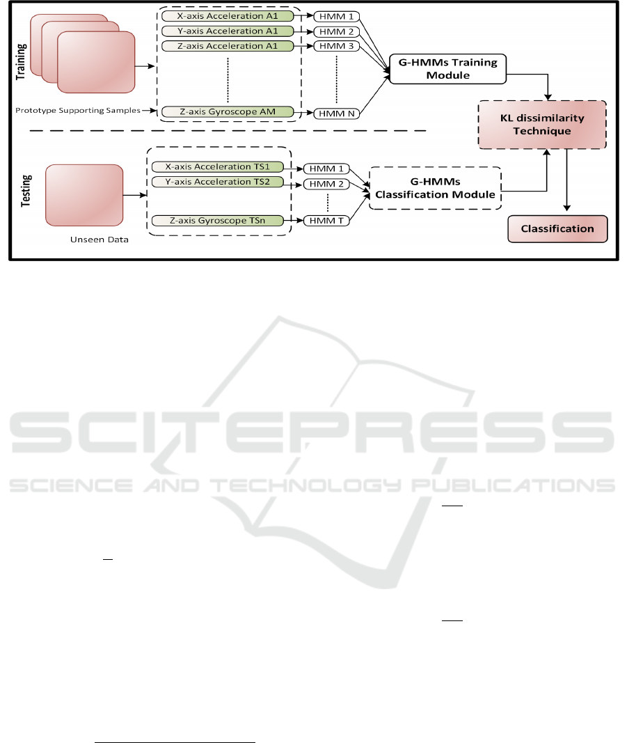
Figure 1: Framework of the proposed model. A* represents the training/prototype samples across all the considered activities.

N is the total number of Hidden Markov Models obtained per-axis across the prototype samples. T S1 - T Sn represent the

per-axis signals for an unseen sample. T is the number of Hidden Markov Models derived from T S1-T Sn which are then

compared against the N prototype HMMs to classify the sample.

Typically, no closed-form solution exists for such

an integration for probability distributions repre-

sented by Hidden Markov Models, so Juang and Ra-

biner (Juang and Rabiner, 1985) proposed a Monte-

Carlo approximation to this integral for comparing

two HMMs (Sahraeian and Yoon, 2011) using a se-

quence of observed symbols. Assume h

and h

are

two HMMs and assume O = o

, . . . , o

is an observa-

tion sequence of length T , then the KL-dissimilarity

between h

and h

can be approximated by the fol-

lowing formula:

k h

) ≈

(logP(O|h

) − log P(O|h

))

(5)

In this context the observation sequence O corre-

sponds to some timeseries ts of a sensor in a cer-

tain axial direction. As can be seen from (5), KL-

divergence is an asymmetric measure. To allow for

more natural (i.e commutative) comparison between

samples, we derive a symmetric form of the KL-

measure as:

symm

k h

) + D

k h

)

(6)

Therefore, given two timeseries ts

and ts

represent-

ing two samples of measurements of some sensor in a

particular axial direction (for example, two samples of

x-axis of the accelerometer) of two activities (which

could be different or the same activity), we compute

the dissimilarity score between ts

and ts

as follows:

1. Let h

be the HMM model built from timeseries

2. Let h

be the HMM model built from timeseries

3. Compute the log-likelihoods logP(ts

logP(ts

), logP(ts

), and logP(ts

4. Compute the KL-divergence D

k h

) as fol-

lows:

k h

) =

|ts

(logP(ts

) − logP(ts

))

(7)

where |ts

| is the length of the timeseries ts.

5. Compute the KL-divergence D

k h

) as fol-

lows:

k h

) =

|ts

(logP(ts

) − logP(ts

))

(8)

where |ts

| is the length of the timeseries ts

6. Compute the symmetric KL-divergence between

and h

as in (6).

7. This last quantity represents the dissimilarity

score between the timeseries ts

and ts

Given two tuples of timeseries corresponding to sen-

sor measurements T S = (ts

, ts

)

and T S

= (ts

, ts

), we need to

compute the dissimilarity measure between these two

samples. To do this, we develop the HMM mod-

els corresponding to these tuples (12 in total, 6 per

sample): H

T S

= (h

, h

) and H

T S

Improved IMU-based Human Activity Recognition using Hierarchical HMM Dissimilarity

705

Figure 2: Figures showing some activities from the E-JUST-

ADL1 dataset (left) and sensor placement from the USC-

HAD dataset (right).

, h

). We use the symmetric KL-

divergence ((6)) to ﬁnd the dissimilarity measure be-

tween every pair of corresponding HMMs in the two

tuples. Then, these dissimilarity scores along the dif-

ferent axes of the two sensors (accelerometer and gy-

roscope) are combined together using summation to

produce a single dissimilarity score between the two

measurement tuples T S and T S

d(T S, T S

) =D

symm

k h

) + D

symm

k h

symm

k h

) + D

symm

k h

symm

k h

) + D

symm

k h

)

(9)

Then, given two samples s and s

consisting of 6-axial

IMU measurements T S and T S

, then the dissimilarity

of s and s

is simply taken to be:

d(s, s

) = d(T S, T S

)

(10)

3.3 Sample-activity Dissimilarity

Given a test sample s corresponding to some unknown

activity and a potential activity A , we compute the

dissimilarity between s and A as follows, considering

that we have a set of dissimilarity scores (obtained

from the previous section) indicating the dissimilarity

between s and each of the prototype samples for A :

d(s, A ) = min{d(s, s

): s

∈ prototype(A )}

(11)

3.4 Classifying Samples

Adopting the notation from the previous section, we

consider that we have computed the sample-activity

dissimilarity scores between the unknown sample s

and each activity A in the dataset. Therefore we have

as many dissimilarity scores as there are activities in

the dataset. Finally, s is assigned to/classiﬁed as the

activity with the minimum dissimilarity score:

∗

= argmin

d(s, A )

(12)

4 EXPERIMENTS

In this section we present the details of the experimen-

tal procedure used to evaluate our proposed method.

4.1 Datasets Considered

In order to demonstrate the efﬁcacy of our proposed

HAR-HMM model, we apply it to two publicly-

available activity recognition datasets: EJUST-ADL-

1 dataset (Gomaa et al., 2017) and USC-HAD (Zhang

and Sawchuk, 2012). The details of these datasets are

provided in Table 1 and Fig 2.

4.2 Experimental Setup

In order to demonstrate the efﬁcacy of our proposed

HAR-HMM model, we perform a number of tests

wherein we alter different parameters of the model

and investigate their effects on its performance. A to-

tal of 4 tests were performed, each test with a different

value for the number of hidden states in the HMMs

ranging from 2 to 5 states as shown in Table2 .

We also tested the performance of the method

in the presence of different sensor combinations as

shown in Table 3.

We adopt the following conﬁguration for all tests

performed:

• In each test we performed a total of 5 experiments.

Results are averaged over those 5 experiments.

• For each activity, the number of samples taken as

the prototypes is 66% of the total number of sam-

ples. The remaining 34% are used for testing.

• For each experiment we produced the following

performance metrics:

– The confusion matrix for all the 14 activities.

– The overall accuracy and its 95% conﬁdence in-

terval.

– The sensitivity and speciﬁcity for each activity.

– The average sensitivity, average speciﬁcity, av-

erage precision, and average F-score.

We also compare our proposed technique against

two other methods: the method presented in (Go-

maa et al., 2017) which requires feature extraction,

and another involving the use of a deep LSTM-

based(Hochreiter and Schmidhuber, 1997) classiﬁer

operating directly on the raw data. This is to give a

sense of the relative performance of our method juxta-

posed against feature extraction-based and other state

of the art sequence modelling-based techniques. The

deep classiﬁer consisted of a single LSTM layer and

ICINCO 2020 - 17th International Conference on Informatics in Control, Automation and Robotics

706

Table 1: Details of Datasets Considered.

Dataset

Number of

Subjects

Activities Sensor Locations Sensors Comments

USC-HAD

(Zhang and

Sawchuk,

2012)

Walk forward, walk left, walk right,

walk up-stairs, walk down-stairs, run

forward, jump, sit on chair, stand, sleep,

elevator up, and elevator down

Front right hip

3D accelerometers, 3D gyro-

scopes

Consists of 12 activities

and 2311 samples in total.

EJUST-

ADL-1

Dataset (Go-

maa et al.,

2017)

Use telephone, Drink from glass, Pour

water, Eat with knife/ fork, Eat with

spoon, Climb/ Descend stairs, Walk,

Get up/Lie down bed, Stand up/ Sit

down chair, Brush teeth, Comb hair

Right wrist only.

3D accelerometers, 3D angular

velocity, 3D rotation, 3D grav-

ity.

14 activities are collected

using an Apple watch Se-

ries 1. Number of samples

is 603.

Table 2: Accuracy of method when used with different

number of HMM hidden states on E-JUST-ADL1 dataset.

No. of Hidden States Accuracy

2 91.9%

3 90.95%

4 89.52%

5 82.46%

Table 3: Accuracy of method when used with different sen-

sor combinations on E-JUST-ADL1 dataset.

Combination Accuracy

Accelerometer 90.9%

Gyroscope 91.62%

Rotation 90.29%

Gravity 91.62%

Accelerometer, Gyroscope, Gravity 90.95%

Accelerometer, Gyroscope, Rotation 87.62%

Acc., Gyro., Rotation, Gravity 91.9%

was trained for 50 epochs with a batch size of 30 sam-

ples. We consider accuracy, sensitivity, speciﬁcity,

precision and F-measure as the metrics of interest. As

stated previously, these metrics are aggregated by av-

eraging over each test run.

We use standard deﬁnitions for the Precision, Re-

call, Speciﬁcity, F-Measure and Accuracy metrics,

described respectively in Equations 13, 14, 15, 16,

and 17. We adopt the following notations:

• N is the number of samples in each activity.

• TP refers to the number of true positives.

• FP is the number of false positives.

• TN is the number of true negatives.

• FN is the number of false negatives.

Precision =

T P

T P + FP

(13)

Sensitivity =

T P

T P + FN

(14)

Speci f icity =

T N

T N + FP

(15)

F − Measure =

2 ∗ Precision ∗ Sensitivity

Precision + Sensitivity

(16)

Accuracy =

T P

(17)

4.3 Discussion

We present the results obtained from our experiments

in Table 4. As described previously, we carry out the

experiments on two publicly-available datasets. We

investigate our proposed technique against a feature

extraction-based technique (Gomaa et al., 2017) and

a deep classiﬁcation technique utilizing a Long Short-

Term Memory (LSTM) network. Note that these re-

sults correspond to a conﬁguration where the HMMs

used have only two hidden states each.

As can be observed from the table, our proposed

method outperforms both of the comparative tech-

niques used on both datasets in all the considered

metrics. Relative to the feature extraction-based

method (denoted as RF in the table), our method

yields better performance as it (by design) respects

the sequential/temporal nature of the data, which

is not necessarily guaranteed with many feature

extraction-based techniques. Additionally, it can be

seen that our method outperforms the deep LSTM-

based classiﬁer (denoted as LSTM in the table). This

can be attributed to the fact that our method is not

only based on sequence-modelling itself, but also

includes similarity-based enhancements in contrast

to the deep classiﬁer. This allows it to leverage the

strengths of both approaches and deliver superior

performance to the deep LSTM-based classiﬁer.

Effect of Sensor Choices. We also investigate the

performance of the method in the presence of differ-

ent sensor combinations. This was done with a view

to discerning the performance of the method in dif-

ferent scenarios, as activity recognition problems may

have different sensor modalities available than the pri-

mary evaluations were performed with. We consid-

ered single modalities and combinations of modali-

ties as shown in Table 3. For clarity of presentation,

we consider only the E-JUST-ADL1 dataset and the

accuracy metric in particular.

It can be seen that the method is able to maintain

consistent performance even with the use of single

Improved IMU-based Human Activity Recognition using Hierarchical HMM Dissimilarity

707

Table 4: A comparison between the proposed HMM-based method, LSTM using raw data, and RF (Gomaa et al., 2017) using

two different public datasets.

Dataset Method Accuracy Sensitivity Speciﬁcity Precision F-Measure

RF 78.5% 70.45% 98.2% 60.5% 65.1%

LSTM 78.57% 72.8% 85.71% 71% 71.88%USC-HAD

HMM 83.95% 83.8% 98.54% 84.36 % 83.49 %

RF 81.64% 82.47% 98.67% 84.6% 83.53%

LSTM 87.19% 78.5% 93.1% 77% 77.74%E-JUST ADL 1

HMM 91.9% 91.4% 99.37% 92.54% 91.64%

sensors. This is due to its use of both sequence

modelling and similarity-based techniques, allowing

the system to both capture the intrinsic dynamics of

the activity as captured by the sensor(s) used and

match samples in that context without explicitly

relying on any particular modality. This indicates the

reliability of the technique in a multitude of possible

deployment scenarios.

Effect of HMM Hidden States. We also experiment

with the number of hidden states in the HMMs used.

This is done to determine a suitable value for this pa-

rameter in the context of the stated task. As stated pre-

viously, the initial set of results (Table 4) indicate the

performance of the method at 2 hidden states. There-

fore we vary the number of hidden states from 3 to 5

for this investigation. Similar to the previous section,

we also consider only the E-JUST-ADL1 dataset for

clarity and the accuracy metric.

Increasing the number of hidden states in the

HMMs has a consistently-increasing detrimental ef-

fect on the method. This can be attributed to the fact

that the underlying processes generating the time se-

ries data per axis are fairly simple, and so increasing

the number of hidden states mischaracterizes the pro-

cess. Therefore, the optimal number of hidden states

per HMM in the proposed method is chosen to be 2.

5 CONCLUSION AND FUTURE

WORK

In this work, we presented an improved HMM-based

technique for human activity recognition based on

IMU-sourced data. We evaluate our technique on

two publicly-available activity recognition datasets

and also compare it against two baseline methods:

one based on traditional feature extraction, and the

other based on a deep LSTM-based technique using

raw data.

The experimental results yielded indicate that the

proposed method is effective for the stated task, as it

outperforms both baseline methods in terms of sev-

eral metrics eg., accuracy, sensitivity, speciﬁcity, pre-

cision, and F-Measure. A potential drawback of the

proposed method is its computational complexity as

it requires the training and retention of a large num-

ber of HMM models. This weakness can be overcome

using parallelization methods such as GPU-based ac-

celeration or similar.

In the future, we intend to investigate the use

of multivariate HMMs to cater for single modalities

rather than individual HMMs per individual axes’ per

modality, as well as multivariate HMMs for all the

axes simultaneously. Furthermore, we intend to inves-

tigate the use of different HMM (dis)similarity mea-

sures on the performance of the proposed method.

ACKNOWLEDGMENT

This work is funded by the Information Technol-

ogy Industry Development Agency (ITIDA), Infor-

mation Technology Academia Collaboration (ITAC)

Program, Egypt – Grant Number (PRP2019.R26.1 - A

Robust Wearable Activity Recognition System based

on IMU Signals).

REFERENCES

Abdu-Aguye, M. G. and Gomaa, W. (2018). Novel ap-

proaches to activity recognition based on vector au-

toregression and wavelet transforms. In 2018 17th

IEEE International Conference on Machine Learning

and Applications (ICMLA), pages 951–954. IEEE.

Abdu-Aguye, M. G. and Gomaa, W. (2019). Competi-

tive feature extraction for activity recognition based

on wavelet transforms and adaptive pooling. In 2019

International Joint Conference on Neural Networks

(IJCNN), pages 1–8.

Abdu-Aguye, M. G. and Gomaa, W. (2019a). Robust hu-

man activity recognition based on deep metric learn-

ing. In n the proceeding of the 16th International Con-

ference on Informatics in Control, Automation and

Robotics (ICINCO).

Abdu-Aguye, M. G. and Gomaa, W. (2019b). Versatl: Ver-

satile transfer learning for imu-based activity recog-

nition using convolutional neural networks. In In

the proceeding of the 16th International Conference

ICINCO 2020 - 17th International Conference on Informatics in Control, Automation and Robotics

708

on Informatics in Control, Automation and Robotics

(ICINCO).

Abdu-Aguye, M. G., Gomaa, W., Makihara, Y., and Yagi, Y.

(2019). On the feasibility of on-body roaming models

in human activity recognition. In ICINCO (1), pages

680–690. SciTePress.

Abdu-Aguye, M. G., Gomaa, W., Makihara, Y., and Yagi,

Y. (2020a). Adaptive pooling is all you need: An em-

pirical study on hyperparameter-insensitive human ac-

tion recognition using wearable sensors, accepted. In

IJCNN. The 2020 International Joint Conference on

Neural Networks.

Abdu-Aguye, M. G., Gomaa, W., Makihara, Y., and Yagi, Y.

(2020b). Detecting adversarial attacks in time-series

data, accepted. In ICASSP. IEEE 45th International

Conference on Acoustics, Speech, and Signal Pro-

cessing.

Ashry, S., Elbasiony, R., and Gomaa, W. (2018). An LSTM-

based Descriptor for Human Activities Recognition

using IMU Sensors. In Proceedings of the 15th In-

ternational Conference on Informatics in Control, Au-

tomation and Robotics - Volume 1: ICINCO, pages

494–501. INSTICC, SciTePress.

Ashry, S. and Gomaa, W. (2019). Descriptors for human

activity recognition. In 2019 7th International Japan-

Africa Conference on Electronics, Communications,

and Computations, (JAC-ECC), pages 116–119.

Ashry, S., Ogawa, T., and Gomaa, W. (2020). Charm-deep:

Continuous human activity recognition model based

on deep neural network using imu sensors of smart-

watch. IEEE Sensors Journal.

Bruno, B., Mastrogiovanni, F., Sgorbissa, A., Vernazza, T.,

and Zaccaria, R. (2013). Analysis of human behavior

recognition algorithms based on acceleration data. In

Robotics and Automation (ICRA), 2013 IEEE Interna-

tional Conference on, pages 1602–1607. IEEE.

Cilla, R., Patricio, M. A., Garc

ıa, J., Berlanga, A., and

Molina, J. M. (2009). Recognizing human activi-

ties from sensors using hidden markov models con-

structed by feature selection techniques. Algorithms,

2(1):282–300.

Elbasiony, R. and Gomaa, W. (2019). A survey on hu-

man activity recognition based on temporal signals of

portable inertial sensors. In International Conference

on Advanced Machine Learning Technologies and Ap-

plications, pages 734–745. Springer.

Feng, Y., Chang, C. K., and Chang, H. (2016). An adl

recognition system on smart phone. In International

Conference on Smart Homes and Health Telematics,

pages 148–158. Springer.

Gaikwad, K. (2012). Hmm classiﬁer for human activ-

ity recognition. Computer Science & Engineering,

2(4):27.

Gomaa, W., Elbasiony, R., and Ashry, S. (2017). Adl clas-

siﬁcation based on autocorrelation function of iner-

tial signals. In Machine Learning and Applications

(ICMLA), 2017 16th IEEE International Conference

on, pages 833–837. IEEE.

Hochreiter, S. and Schmidhuber, J. (1997). Long short-term

memory. Neural computation, 9(8):1735–1780.

Juang, B. . and Rabiner, L. R. (1985). A probabilistic dis-

tance measure for hidden markov models. AT T Tech-

nical Journal, 64(2):391–408.

Kabir, M. H., Hoque, M. R., Thapa, K., and Yang, S.-

H. (2016). Two-layer hidden markov model for hu-

man activity recognition in home environments. In-

ternational Journal of Distributed Sensor Networks,

12(1):4560365.

Karaman, S., Benois-Pineau, J., Dovgalecs, V., M

egret,

R., Pinquier, J., Andr

e-Obrecht, R., Ga

estel, Y., and

Dartigues, J.-F. (2014). Hierarchical hidden markov

model in detecting activities of daily living in wear-

able videos for studies of dementia. Multimedia tools

and applications, 69(3):743–771.

Khan, A. M., Lee, Y.-K., Lee, S. Y., and Kim, T.-

S. (2010). A triaxial accelerometer-based physical-

activity recognition via augmented-signal features and

a hierarchical recognizer. IEEE transactions on infor-

mation technology in biomedicine, 14(5):1166–1172.

Kreil, M., Sick, B., and Lukowicz, P. (2014). Dealing

with human variability in motion based, wearable ac-

tivity recognition. In 2014 IEEE International Con-

ference on Pervasive Computing and Communication

Workshops (PERCOM WORKSHOPS), pages 36–40.

IEEE.

Lara, O. D. and Labrador, M. A. (2012). A survey

on human activity recognition using wearable sen-

sors. IEEE communications surveys & tutorials,

15(3):1192–1209.

Machado, I. P., Gomes, A. L., Gamboa, H., Paix

ao, V.,

and Costa, R. M. (2015). Human activity data

discovery from triaxial accelerometer sensor: Non-

supervised learning sensitivity to feature extraction

parametrization. Information Processing & Manage-

ment, 51(2):204–214.

Mohammed, S. A. and Gomaa, W. (2016). Exploration of

unknown map for gas searching and picking up ob-

jects using khepera mobile robots. In ICINCO (2),

pages 294–302.

Mohammed, S. A. and Gomaa, W. (2017). Exploration of

unknown map for safety purposes using wheeled mo-

bile robots. In ICINCO (2), pages 359–367.

Sahraeian, S. M. E. and Yoon, B. (2011). A novel low-

complexity hmm similarity measure. IEEE Signal

Processing Letters, 18(2):87–90.

Zhang, M. and Sawchuk, A. A. (2012). Usc-had: a daily ac-

tivity dataset for ubiquitous activity recognition using

wearable sensors. In Proceedings of the 2012 ACM

Conference on Ubiquitous Computing, pages 1036–

1043. ACM.

Improved IMU-based Human Activity Recognition using Hierarchical HMM Dissimilarity

709