Damage Detection and Diagnosis for Offshore Wind Foundations

Bryan Puruncajas

1,2 a

, Yolanda Vidal

2 b

and Christian Tutiv

1 c

Mechatronics Engineering, Faculty of Mechanical Engineering and Production Science (FIMCP),

Escuela Superior Polit

ecnica del Litoral (ESPOL), Guayaquil, Ecuador

Department of Mathematics, Control, Modeling, Identiﬁcation and Applications (CoDAlab),

Universitat Polit

ecnica de Catalunya (UPC), 08019 Barcelona, Spain

Keywords:

Structural Health Monitoring, Offshore Wind Turbine, Structural Vibration, Data-driven, Convolutional

Neural Network.

Abstract:

Structural health monitoring for wind turbines (WT) in remote locations, as offshore, is crucial (Presencia

and Shaﬁee, 2018). Offshore wind farms are increasingly realized in water depths beyond 30 meters, where

lattice foundations (as jacket-type) are a highly competitive substructure type (Moulas et al., 2017). In this

work, a methodology for the diagnosis of structural damage in jacket-type foundations is stated by means

of a small-scale structure -an experimental laboratory tower modeling an offshore-ﬁxed jacket-type WT. In

the literature, a lot of methodologies for damage detection can be found (Li et al., 2015). Among them,

the vibration-based methods are one of the most proliﬁc ones. However, they are, primarily, focused on

the case of measurable input excitation and vibration response signals, with only few recent studies focused

on the vibration–response–only case, the importance of which stems from the fact that in some applications

the excitation cannot be imposed and often is not measurable. This work aims to contribute in this area, as

the vibration excitation is given by the wind and analyzed by a convolutional neural network (CNN), with a

classiﬁcation accuracy result of 93 %.

1 INTRODUCTION

Wind energy is one of the best sources of fuel, as it

is clean, relatively cheap and inexhaustible. In or-

der to increase the energy produced by these means,

more offshore wind farms have been installed (Selot

et al., 2018). Given the location of wind turbines and

the sea conditions, new problems related to inspec-

tion, maintenance and repair work arise (Zhang et al.,

2016). To reduce logistics and maintenance costs, as

well as to minimize turbine downtime, it is crucial that

wind turbines are continuously monitored (Breteler

et al., 2015). In particular, a structural health moni-

toring system (SHM) is needed to verify the state of

the structure to guarantee its correct operation and de-

termine whether the wind turbine needs some mainte-

nance.

There are different types of WT foundations, see

Figure 1, depending on the depth at which the WT

will be installed. In general, monopiles are used in

https://orcid.org/0000-0002-2194-6853

https://orcid.org/0000-0003-4964-6948

https://orcid.org/0000-0001-6322-4608

installations at depths below 15 meters, gravity foun-

dations are preferred when depth is less than 30 me-

ters, and jackets are the option used for greater depths,

(Klijnstra et al., 2017). This work proposes a com-

plete methodology for SHM (damage detection and

classiﬁcation) of a jacket-type foundation tested in a

laboratory offshore-ﬁxed wind turbine model. The

only excitation of the WT is assumed to be given

by wind turbulence, so the input excitation is as-

sumed to be unknown. The proposed method is vi-

bration–response–only and can be summarized in the

following steps: (i) the wind excitation is simulated

as a Gaussian white noise and the data coming from

the WT is collected using a set of accelerometers; (ii)

the raw data are pre-processed and converted into im-

ages using as many channels as sensors; (iii) a con-

volutional neural network is stated as a classiﬁer. The

damage detection strategy is applied to different types

of predeﬁned damage. The obtained results demon-

strate the reliability of the proposed approach.

Puruncajas, B., Vidal, Y. and Tutivén, C.

Damage Detection and Diagnosis for Offshore Wind Foundations.

DOI: 10.5220/0009886101810187

In Proceedings of the 17th International Conference on Informatics in Control, Automation and Robotics (ICINCO 2020), pages 181-187

ISBN: 978-989-758-442-8

181

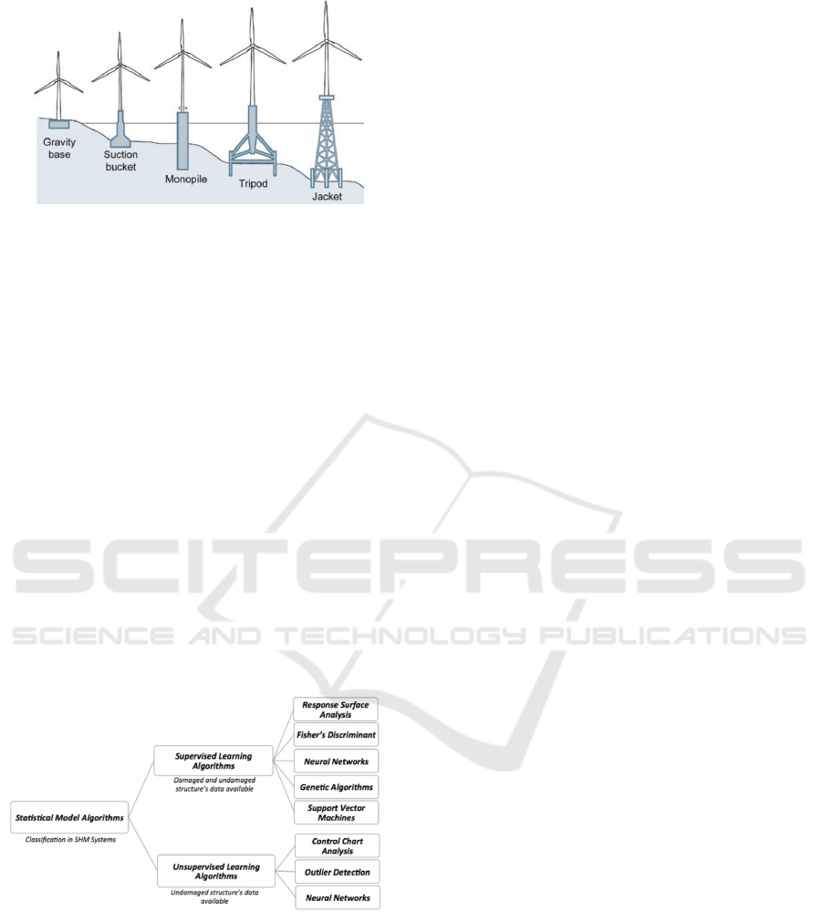
Figure 1: Types of foundations (Association et al., 2012).

2 RELATED WORK

The ﬁrst SHM study dates back 50 years ago. In

70s and 80s, the oil industry faced the problem of

identifying damage in offshore platforms (Martinez-

Luengo et al., 2016). They struggled to develop meth-

ods based on identifying vibrations to locate the dam-

age. At the same time, the aerospace community

began investigating the use of vibration-based strate-

gies. This approach has continued with the current

research of the National Aeronautics and Space Ad-

ministration (Seshadri et al., 2016). Currently, SHM

has been developed in the ﬁelds of civil aviation in-

dustry (Khan et al., 2014) and civil structures (Song

et al., 2017). SHM is highly multidisciplinary, and

advances in other areas of study can probably be re-

cruited for SHM’s progress.

Figure 2 shows a general classiﬁcation for differ-

ent types of strategies for SHM.

Figure 2: Algorithms classiﬁcation (Martinez-Luengo et al.,

2016).

The methodology implemented in this work is based

on supervised learning algorithms. Speciﬁcally on

neural networks (NN), which are recently used in

structural health monitoring to identify, locate, and

quantify damage in different types of structures (Liu

et al., 2017). One of the best-known deep NNs is

the convolutional neural network (CNN). A CNN is

commonly used to recognize objects in images given

their ability to exploit spatial or temporal correlation

in the data (Albawi et al., 2017). A CNN has multi-

ple layers; including fully connected layers, grouping

layers, convolutional and nonlinear layers. Fully con-

nected layers and convolutional layers have parame-

ters, however non-linearity and grouping layers have

no parameters.

Some research has been conducted related to CNN

in the ﬁeld of SHM. For example, (Tabian et al., 2019)

proposes to collect impact waves using piezoelectric

sensors (PZT) to detect and locate impacts (this ap-

proach was tested on a rigid panel). Another method

with piezoelectric sensors is used in (De Oliveira

et al., 2018), where the signals from the sensors are

transformed to RGB images. A different study fo-

cused on transfer learning (TL) techniques to train

with discrete histogram data (compressed data) is pre-

sented in (Azimi and Pekcan, 2019). Their results in-

dicate that deep TL can be effectively implemented

for SHM of similar structural systems with different

types of sensors. However, these previous works used

known-input vibration signals. In this work, it is pro-

posed to use CNN for damage diagnosis in wind tur-

bines foundations by using only vibration-response

data. The strategy consists on transforming the vi-

bration signals into images (with as many channels as

sensors), and then classify the images with its corre-

sponding structural state label.

3 EXPERIMENTAL SET-UP

The general overview of the experimental testbed is

given in Figure 3 and explained as follows.

The experiment starts with a white noise signal

given by the function generator. This signal is am-

pliﬁed and passed to the inertial shaker. This is re-

sponsible for generating vibrations (similar to those

produced by gusts of wind on the blades) to the lab-

oratory tower structure. The shaker is placed at the

upper part of the structure, thus simulating the nacelle

mass. The simulation of different wind speed is also

simulated with this shaker, by changing the amplitude

of the input electrical signal. In particular, multiply-

ing it by the factors 0.5, 1, 2, and 3. Finally, the struc-

ture is monitored by 8 triaxial accelerometers which

are connected to the data acquisition system. Thus,

data from 24 sensors is collected. The nomenclature

used for each sensor is given in Table1.

The real structure used in this work is a tower model.

From Figure 3 (offshore platform) it can be seen the

components of the structure: jacket, tower and na-

celle. As a whole, this structure is 2.7 m high. The

tower is composed of three sections joined with bolts.

ICINCO 2020 - 17th International Conference on Informatics in Control, Automation and Robotics

182

Figure 3: General overview of the experimental testbed.

Table 1: Nomenclature used to refer to each available sen-

sor. Note that i = 1,...,8, as there are eight accelerometers.

Sensor

Acceleration in x-direction for accelerometer number i

Acceleration in y-direction for accelerometer number i

Acceleration in z-direction for accelerometer number i

The jacket is composed with several sections, all of

them joined with bolts, with a torque of 12 Nm. The

different studied damages are introduced in one of

these sections. The top piece (representing the na-

celle) is 1 m long and 0.6 m width.

Two types of damage are introduced at the jacket

support: a 5 mm crack in one of the bars; and loos-

ening one of the bolts in the jacket. Also a healthy

replica of the studied bar has been considered, as the

proposed strategy should be able to detect and clas-

sify the studied types of damage, but also be robust

to the replacement of one bar by a new healthy one

(avoiding false alarms).

4 DAMAGE DETECTION AND

CLASSIFICATION

METHODOLOGY

The proposed SHM methodology is composed by the

following steps. First, the data is collected from

the experiment and reshaped. Second, the data is

pre-processed in order to obtain a data set of multi-

channel images. Third, a CNN with 24 channel in-

puts is designed and trained for classiﬁcation of the

different types of damage.

4.1 Data Collection and Reshape

The time window for each experimental test is 60 sec-

onds with a sampling frequency of approximately 257

Hz. Thus, each experiment obtains 16517 data mea-

surements from each of the 24 sensors. In this work,

a total of 25 experimental tests are conducted for each

different white noise amplitude. In particular:

• 10 tests with the original bar.

• 5 tests with the replica bar.

• 5 tests with a 5 mm crack damaged bar.

• 5 tests with an unlocked bolt damage.

That is 100 experiments in total, as there are 25 ex-

periments for each one of the 4 different considered

white noise amplitudes. Given the k-th experimen-

tal test, the data is initially stored in a matrix Y

(k)

∈

16517×24

(R) such that:

(k)







(k)

1,1

(k)

1,2

· · · y

(k)

1,24

(k)

2,1

(k)

2,2

· · · y

(k)

2,24

(k)

16517,1

(k)

16517,2

· · · y

(k)

16517,24







, (1)

where the number of rows is given by the number of

time stamps in each experimental test and the number

of columns is equal to the number of sensors. Note

that data in the ﬁrst, second and third columns (A

) come from accelerometer 1; fourth, ﬁfth and sixth

columns are related to the second accelerometer, and

so on until the last accelerometer.

To convert the data into images, the dimensions

of matrix Y

(k)

have been chaned. In particular, the

data coming from the k-th experimental test, Y

(k)

, is

reshaped to a matrix Z

(k)

∈ M

64×(256·24)

(R), that is a

matrix with 64 rows and 256 · 24 = 6144 columns as

detailed in Table 2. Note that the last samples (from

16385 to 16517) of each sensor are discarded.

4.2 Signal to Image Conversion

The damage diagnosis method converts time-domain

signals, from the 24 measured sensors, into 2D gray

level images to exploit texture information from the

converted images. The data conversion process is in-

spired in reference (Ru

ız et al., 2018) but here it is

enhanced by using multi-channel images.

Damage Detection and Diagnosis for Offshore Wind Foundations

183

In particular, ﬁrst the values in matrix Z

(k)

are

scaled between 0 and 255. This will allow an easy

conversion into gray scale images. The image size

used for signal to image conversion is 16 × 16 (256

pixels) with 24 channels (one per sensor) and it is con-

structed as follows. For each sensor (different blocks

of matrix Z

(k)

, see Table 2) the ﬁrst 16 data-points

determine the ﬁrst row of the gray-scale image; im-

mediately after, the next 16 data points determine the

second row and ﬁnally the data points 240 to 256 de-

termine the last row of the image. That is, each row

of matrix Z

(k)

is converted to 24 gray-scale images

(one per sensor) with size 16 × 16. In fact, in order to

apply convolutional neural networks, it is proposed to

shape these data as one image with 24 channels (one

per sensor), similarly to RGB images (with 3 chan-

nels). Note that, considering that the sampling time

is 1/257 seconds, each image contains approximately

one second of data from all the sensors, which ensures

to capture all the system dynamics. The total number

of images in the data set is 6400, as there are 64 im-

ages coming from each one of the 100 experiments.

Figure 4 shows one of the multi-channel images.

Figure 4: Multi-channel gray-scale image corresponding to

the 24 sensors (size 16 × 16).

4.3 Convolutional Neural Network

(CNN)

The next step of the proposed damage diagnosis

method is to use a convolutional neural network

(CNN) in order to detect and classify the damage

state. The input data to the CNN are the multi-channel

gray-scale images obtained from the signal-to-image

conversion explained in the previous section.

The proposed CNN architecture is shown in Fig-

ure 5 and the most signiﬁcant characteristics are

given in Table 3. Brieﬂy explained, ﬁrst, the gray-

scale images (16 × 16 × 24) are applied to the ﬁrst

convolutional module. This module is composed of

32 ﬁlters (kernel 5 × 5) and padding of 1, resulting

in an output size of 14 × 14 × 32. Next, the second

and the third convolutional layers have the same ker-

nel and same padding, resulting in an output size of

12 × 12 × 64 and 10 × 10 × 32, respectively. Then, a

fully connected layer of size 1 × 1 × 4 is connected

and ﬁnally, the softmax layer outputs the predicted

structural condition. The data set is split into 70% for

training and 30% for validation.

The parameters have been optimized with Adam,

which is an adaptive learning rate method. This

method is easy to implement, is computationally ef-

ﬁcient, has few memory requirements, and hyper-

parameters have intuitive interpretations and gener-

ally require little tuning (Kingma and Ba, 2014). The

selected hyper-parameter values are an initial learning

rate of α

= 0.01, a gradient decay factor of β

= 0.9,

a squared gradient decay factor of β

= 0.992, and a

value ε = 10

−7

. Moreover, the learning rate is drop

every 2 epochs by multiplying with factor 0.5, and ﬁ-

nally, L2 regularization with λ = 10

−6

is employed.

Finally, a ﬂowchart of the proposed approach is

shown in Figure 6. When a WT has to be diagnosed,

the accelerometers data are scaled, reshaped and con-

verted into gray-scale images that are fed into the al-

ready trained CNN. A classiﬁcation is obtained to pre-

dict the condition of the structural state.

5 RESULTS

A comprehensive decomposition of the error between

the true classes and the predicted classes is shown by

means of the so-called confusion matrix in Table 4.

Each row represents the instances in a true class while

each column represents the instances in a predicted

class. The ﬁrst row is labeled as 1 and corresponds to

Table 2: Data reshape for each experimental test k = 1,...,100.

Sensor 1 Sensor 2 . . . Sensor 24

(k)







(k)

1,1

· · · y

(k)

256,1

(k)

257,1

· · · y

(k)

512,1

(k)

16129,1

· · · y

(k)

16384,1

(k)

1,2

· · · y

(k)

256,2

(k)

257,2

· · · y

(k)

512,2

(k)

16129,2

· · · y

(k)

16384,2

· · ·

(k)

1,24

· · · y

(k)

256,24

(k)

257,24

· · · y

(k)

512,24

(k)

16129,24

· · · y

(k)

16384,24







ICINCO 2020 - 17th International Conference on Informatics in Control, Automation and Robotics

184

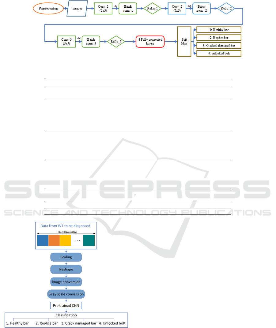
Figure 5: Architecture of the developed CNN.

Table 3: Detailed characteristics of each CNN layer.

Layer Ouput size Parameters

Input

16×16×24 images

16×16×24 -

Convolution#1

32 ﬁlters of size 5×5×24 with padding [1 1 1 1]

14×14×32

Weight 5×5×24×32

Bias 1×1×32

Batch Normalization#1 14×14×32

Offset 1×1×32

Scale 1×1×32

ReLu#1 14×14×32 -

Convolution#2

64 ﬁlters of size 5×5×24 with padding [1 1 1 1]

12×12×64

Weight 5×5×24×64

Bias 1×1×64

Batch Normalization#2 12×12×64

Offset 1×1×64

Scale 1×1×64

ReLu#2 12×12×64 -

Convolution#3

32 ﬁlters of size 5×5×24 with padding [1 1 1 1]

10×10×32

Weight 5×5×24×32

Bias 1×1×32

Batch Normalization#3 10×10×32

Offset 1×1×32

Scale 1×1×32

ReLu#3 10×10×32 -

Fully connected layer#1 1×1×4

Weight 4×3200

Bias 1×1

Softmax - -

classoutput - -

Figure 6: Flowchart to illustrate how the proposed SHM

strategy is applied when a WT has to be diagnosed.

the original healthy bar, the next rows are labeled with

2, 3 and 4, corresponding to the replica bar, the crack

damaged bar and the unlocked bolt, respectively.

After 64 epochs of training on a laptop running

Windows 10 with an Intel Core i7-9750H, 16 GB of

RAM and a graphic card (GeForce RTX 2060) of 6

GB of GPU, the obtained overall accuracy perfor-

mance is 93%. A high true positive rate (TPR) of

94.04% for the original healthy bar is reached, fol-

lowed by a 93.06% of TPR for the replica bar. The

results for the crack damaged bar and unlocked bolt

are 92.23% and 91.88% respectively. Furthermore,

the obtained average recall is 92.8%, the average pre-

cision is 92.3% and, ﬁnally, a F1-score of 92.55% is

achieved.

Figure 7 shows the accuracy and loss curves dur-

ing the CNN training. Note that the training data set

reached 100% accuracy while the validation set only

obtained an accuracy of 93%. This variance could be

improved with more data. However, the results con-

ﬁrm the viability of the proposed methodology.

5.1 Conclusions

This work proposes a SHM methodology for jacket-

type wind turbine foundations using only accelerome-

ter information. The strategy is validated experimen-

tally for different types of predeﬁned damages on a

Damage Detection and Diagnosis for Offshore Wind Foundations

185

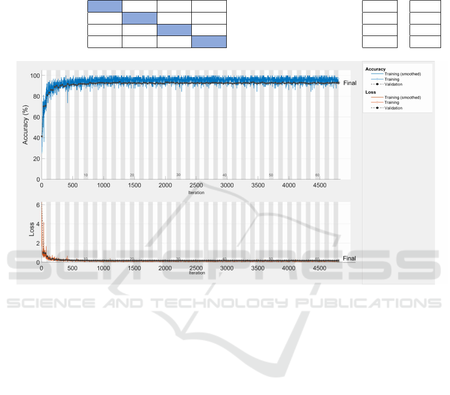
Table 4: Validation set confusion matrix. The ﬁrst row is labeled as 1 and corresponds to the original healthy bar, the next

rows are labeled with 2, 3 and 4, corresponding to a replica bar, crack damaged bar and unlocked bolt, respectively. True

positive rate (TPR) and false negative rate (FNR) of each class are given.

Predicted class TPR FNR

True class

94.04 2.14 1.99 1.83 1. Healthy bar 94.04 5.96

3.47 93.06 3.15 0.32 2. Replica bar 93.06 6.94

0.65 2.91 92.23 4.21 3. Crack damaged bar 92.23 7.77

3.75 0.63 3.75 91.88 4. Unlocked bolt 91.88 8.13

Figure 7: Accuracy and loss curves. The accuracy is represented by blue lines, the loss is represented by orange lines and the

validation results are represented by black dotted lines.

small-scale laboratory tower. In a nutshell, this work

applies the idea to represent time domain accelera-

tion signals to multi-channel gray-scale images and

then utilize convolutional neural networks for classi-

ﬁcation of the different structural states. The obtained

results, with an overall accuracy of 93%, demonstrate

the viability of the proposed approach. Future work

will deal with data augmentation in order to reduce

the validation error with respect to the train set error.

REFERENCES

Albawi, S., Mohammed, T. A., and Al-Zawi, S. (2017).

Understanding of a convolutional neural network. In

2017 International Conference on Engineering and

Technology (ICET), pages 1–6. IEEE.

Association, W. S. et al. (2012). Steel solutions in the green

economy-wind turbines. Brussels, Belgium.

Azimi, M. and Pekcan, G. (2019). Structural health moni-

toring using extremely compressed data through deep

learning. Computer-Aided Civil and Infrastructure

Engineering.

Breteler, D., Kaidis, C., Tinga, T., and Loendersloot, R.

(2015). Physics based methodology for wind turbine

failure detection, diagnostics & prognostics. EWEA

2015 Annual Event.

De Oliveira, M. A., Monteiro, A. V., and Vieira Filho, J.

(2018). A new structural health monitoring strategy

based on pzt sensors and convolutional neural net-

work. Sensors, 18(9):2955.

Khan, A. A., Zafar, S., Khan, N., and Mehmood, Z. (2014).

History current status and challenges to structural

health monitoring system aviation ﬁeld. Journal of

Space Technology, 4(1):67–74.

Kingma, D. P. and Ba, J. (2014). Adam: A

method for stochastic optimization. arXiv preprint

arXiv:1412.6980.

Klijnstra, J., Zhang, X., van der Putten, S., and R

ockmann,

C. (2017). Technical risks of offshore structures.

In Aquaculture Perspective of Multi-Use Sites in the

Open Ocean, pages 115–127. Springer, Cham.

Li, D., Ho, S.-C. M., Song, G., Ren, L., and Li, H.

(2015). A review of damage detection methods for

wind turbine blades. Smart Materials and Structures,

24(3):033001.

Liu, W., Wang, Z., Liu, X., Zeng, N., Liu, Y., and Alsaadi,

F. E. (2017). A survey of deep neural network ar-

ICINCO 2020 - 17th International Conference on Informatics in Control, Automation and Robotics

186

chitectures and their applications. Neurocomputing,

234:11–26.

Martinez-Luengo, M., Kolios, A., and Wang, L. (2016).

Structural health monitoring of offshore wind tur-

bines: A review through the statistical pattern recog-

nition paradigm. Renewable and Sustainable Energy

Reviews, 64:91–105.

Moulas, D., Shaﬁee, M., and Mehmanparast, A. (2017).

Damage analysis of ship collisions with offshore wind

turbine foundations. Ocean Engineering, 143:149–

162.

Presencia, C. E. and Shaﬁee, M. (2018). Risk analysis of

maintenance ship collisions with offshore wind tur-

bines. International Journal of Sustainable Energy,

37(6):576–596.

ız, M., Mujica, L. E., Alf

erez, S., Acho, L., Tutiv

en, C.,

Vidal, Y., Rodellar, J., and Pozo, F. (2018). Wind tur-

bine fault detection and classiﬁcation by means of im-

age texture analysis. Mechanical Systems and Signal

Processing, 107:149–167.

Selot, F., Fraile, D., and Brindley, G. (2018). Offshore wind

in europe-key trends and statistics 2018.

Seshadri, B. R., Krishnamurthy, T., and Ross, R. W. (2016).

Characterization of aircraft structural damage using

guided wave based ﬁnite element analysis for in-ﬂight

structural health management.

Song, G., Wang, C., and Wang, B. (2017). Structural health

monitoring (shm) of civil structures.

Tabian, I., Fu, H., and Sharif Khodaei, Z. (2019). A convo-

lutional neural network for impact detection and char-

acterization of complex composite structures. Sen-

sors, 19(22):4933.

Zhang, J., Fowai, I., and Sun, K. (2016). A glance at off-

shore wind turbine foundation structures. Brodograd-

nja: Teorija i praksa brodogradnje i pomorske

tehnike, 67(2):101–113.

Damage Detection and Diagnosis for Offshore Wind Foundations

187