Predicting the Environment of a Neighborhood: A Use Case for France

Nelly Barret

1 a

, Fabien Duchateau

1 b

, Franck Favetta

1 c

and Loïc Bonneval

LIRIS UMR5205, Université de Lyon, UCBL, Lyon, France

Centre Max Weber, Université de Lyon, France

Keywords:

Data Science, Machine Learning, Data Integration, Environment Prediction, Neighbourhood Study.

Abstract:

Notion of neighbourhoods is critical in many applications such as social studies, cultural heritage manage-

ment, urban planning or environment impact on health. Two main challenges deal with the deﬁnition and

representation of this spatial concept and with the gathering of descriptive data on a large area (country). In

this paper, we present a use case in the context of real estate search for representing French neighbourhoods in

a uniform manner, using a few environment variables (e.g., building type, social class). Since it is not possible

to manually classify all neighbourhoods, our objective is to automatically predict this new information.

1 INTRODUCTION

Data science is a recent discipline which aims at ex-

ploiting data for producing new knowledge. It is at

the crossroads of data management, statistics, ma-

chine learning and visualization. It is also usually

associated with Big Data, as the amount of avail-

able information grows exponentially every year. Two

main tasks for data scientists involve data preparation

and prediction on observations through the detection

of patterns (Dhar, 2013). Numerous application do-

mains beneﬁt from this discipline: health, transport,

environment, media, biology, astronomy – to only cite

a few. Relating data science experiences enable to

demonstrate the feasibility of such projects, the im-

portance of main tasks such as data preparation and

the quality of predictive models.

In this paper, we are interested in the study of ter-

ritories, a long-standing research topic which has re-

cently gained more attention with the emergence of

smart cities (Caragliu et al., 2011). Many works in

Digital Humanities aim at studying neighbourhoods,

since this spatial delimitation enables the detection of

local trends (Delmelle, 2015). Our work is also re-

lated to neighbourhoods in the context of real estate

search, especially when moving to a new city (e.g.,

job transfer). Indeed, people who look for renting or

buying an accommodation may not necessarily have

https://orcid.org/0000-0002-3469-4149

https://orcid.org/0000-0001-6803-917X

https://orcid.org/0000-0003-2039-3481

prior knowledge about their future city or area. Thus

it is difﬁcult to choose a suitable neighbourhood to

live in. One may look for a vibrant neighbourhood

with many pubs while other may prefer a quiet res-

idential area close to schools and parks. Although

several works were designed to tackle this challenge

(Yuan et al., 2013; Tang and Sangani, 2015; Le Fal-

her et al., 2015; Barret et al., 2019), most of them are

either dedicated to a few cities, or the predicted cri-

teria are limited to have a clear understanding of the

neighbourhood. Thus, our objective is to character-

ize neighbourhoods according to a few criteria such

as social class (e.g., lower, middle) or morphological

position (e.g., urban, rural).

Our paper describes a use case for predicting

the environment of a neighbourhood in France. To

reach this goal, the main challenging processes of data

science are required. We ﬁrst introduce related work

(Section 2). Next, we present our method for mod-

elling, collecting and integrating data about neigh-

bourhoods (Section 3), and we describe our choices

for prediction (Section 4). In Section 5, preliminary

experiment results are detailed and analysed. Section

6 concludes and highlights perspectives.

2 RELATED WORK

Multiple projects focus on studying neighbourhoods.

A recent paper shows that the deﬁnition of the area

perceived as neighbourhood is different according to

the point of view (e.g., administrative, from locals,

294

Barret, N., Duchateau, F., Favetta, F. and Bonneval, L.

Predicting the Environment of a Neighborhood: A Use Case for France.

DOI: 10.5220/0009885702940301

In Proceedings of the 9th International Conference on Data Science, Technology and Applications (DATA 2020), pages 294-301

ISBN: 978-989-758-440-4

economic), and consequently, its delimitation are not

completely ﬁxed (Bonneval et al., 2019).

Gathering data collection is a critical issue and

most projects or application do not detail this process.

The website DataFrance

integrates data from diverse

sources, such as indicators provided by the National

Institute of Statistics (INSEE), geographical informa-

tion from the National Geographic Institute (IGN) and

surveys from newspapers for prices (L’Express).

Comparison between neighbourhoods is performed

in many works. Cosine similarity and Jaccard metric

are the most used methods to perform such compari-

son (Yu et al., 2016). They enable a direct computa-

tion of the similarity degree between two spatial areas

described as vectors of values. For instance, authors

of HoodSquare exploit Foursquare check-ins, place

types (e.g., restaurant, ofﬁce, entertainment) and tem-

poral information to detect neighbourhood boundaries

and similar areas (Zhang et al., 2013). The work from

Le Falher et al. discovers similar neighbourhoods be-

tween cities (Le Falher et al., 2015). To reach this

goal, they use classiﬁcation algorithms applied on so-

cial networks data.

Prediction and recommendation are main objec-

tives when working with neighbourhoods. The study

from Tang et al. compare Airbnb announcements in

San Francisco to determine their price and neighbour-

hood (Tang and Sangani, 2015). The VizLIRIS appli-

cation uses machine learning to detect similar areas

in France, which is convenient when moving to a new

location (Barret et al., 2019). Besides, it includes a

grouping functionality for displaying similar neigh-

bourhoods in a selected area or city. In South Ko-

rea, ﬁnding the most relevant neighbourhood and ac-

commodation is based on similar user proﬁles (Yuan

et al., 2013). For instance, the household composi-

tion and the distance from home to work are part of

these proﬁles. Case-based reasoning is performed to

associate a new proﬁle to existing ones, and thus to

adjust recommendations. Finally, the objective of the

Livehoods project is to deduce city’s dynamics from

its resident’s behaviour (Cranshaw et al., 2012). Ex-

periments in Pittsburgh, using 18 million check-ins

and validated by 27 interviews, have conﬁrmed that

municipal districts have a different shape than a rep-

resentation based on their usage.

Several applications, which are closer to the context

of this paper, produce neighbourhood recommenda-

tions. The following list is non exhaustive and centred

on France. Kelquartier

describes the main French

cities using quantitative criteria (e.g., average income,

http://datafrance.info/

http://www.kelquartier.com/

density of schools, density of shops). Home in Love

vivroù

and Cityzia

are more oriented towards users

as they take into account itineraries (e.g., from and

to work) or life style. All aim at recommending the

most relevant neighbourhood(s). Finally, ville-ideale

is a collaborative website for evaluating French cities.

Users give a score (out of 10) for each of the ten cat-

egories, from healthcare to security or culture. Al-

though not at a ﬁne-grained level, user comments may

include mentions of neighbourhood, which is useful

for a (manual) estimation of its quality.

Positioning. Our contribution differs from existing

works on several points. First, some works are lim-

ited to a few cities, which is not possible in a con-

text of job transfer. Our approach should work for

a whole country. Although exploiting user proﬁles

is interesting, they are not always available. Relying

on social data implies prior analysis in order to avoid

bias (e.g., over-represented class of people or activ-

ities). Most approaches focus on life quality while

our goal is to describe environment. Finally, neigh-

bourhoods may be described using tens or hundreds

of criteria, which makes it difﬁcult both for obtaining

a simple representation of the area and for explain-

ing or proving justiﬁcations about recommendations.

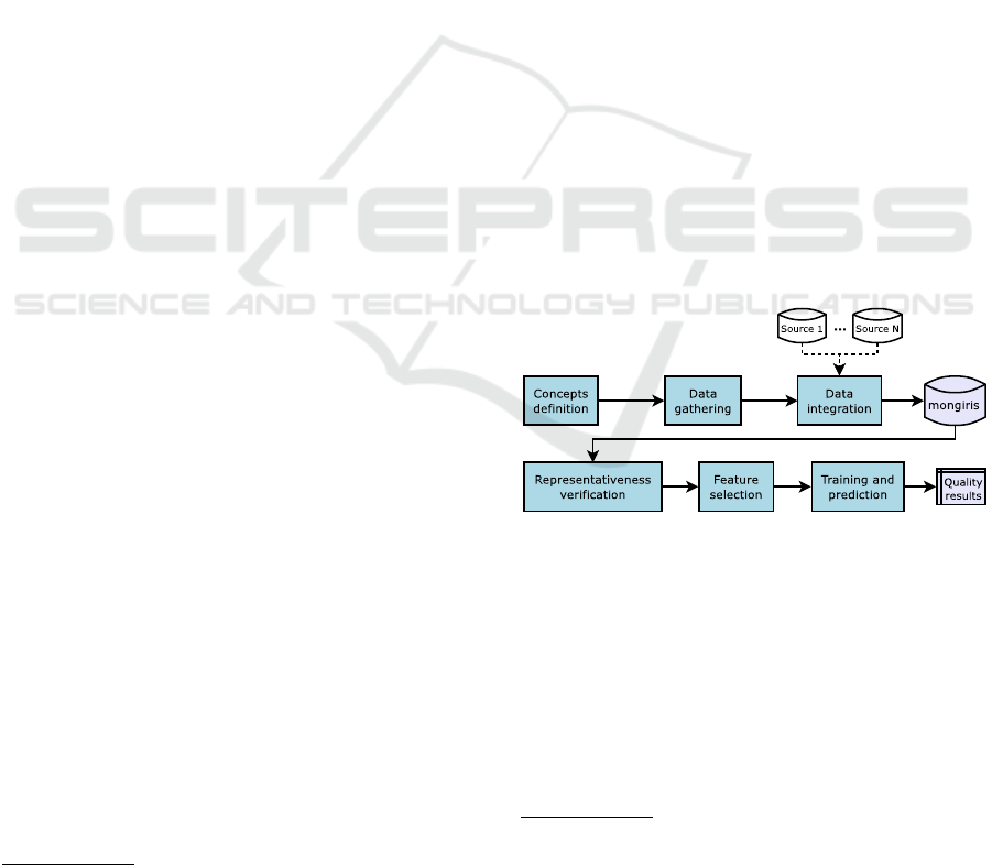
Figure 1 summarizes the main steps of our proposi-

tion, from data preparation (concepts deﬁnition, data

gathering and integration, presented in Section 3) and

prediction (representativeness, feature selection and

algorithm execution, described in Section 4).

Figure 1: The main steps of our approach.

3 DATA PREPARATION

In his study about data science, Donoho estimates

that data scientists spend 80% effort to prepare data

(Donoho, 2017). Indeed this process consists in de-

termining the main concepts to be used, gathering and

extracting information that describe these concepts

and integrating them into a single database.

http://homeinlove.fr/

http://www.vivrou.com/

http://www.cityzia.fr/

http://www.ville-ideale.fr/

Predicting the Environment of a Neighborhood: A Use Case for France

295

3.1 Concepts Deﬁnition

The ﬁrst concept that needs to be deﬁned is the neigh-

bourhood (Bonneval et al., 2019). The deﬁnition of

this spatial object clearly depends on the point of

view: administrative people could refer to a voting

or cadastral deﬁnition while geographers could rely

on natural borders. Residents also have their own

boundaries in mind and an economic point of view

can span over several neighbourhoods. Given these

constraints, we have chosen to use IRIS

as neigh-

bourhoods, i.e., small division units of the French

territory deﬁned for statistical purposes (with about

2,000 residents, thus mainly small-sized in cities and

wider in rural areas). They are deﬁned by INSEE, the

National Institute of Statistics, which ensures a cer-

tain data quality and frequent updates. In addition to

their ofﬁcial nature, the main advantage is that each

IRIS includes many indicators such as the average in-

come, the number of bakeries, the number of build-

ings built before 1950 or the percentage of residents

per socio-economic category. These indicators could

serve as features for the prediction part. There are

around 49,800 IRIS in France, with an average of 550

indicators per IRIS. In the rest of this paper, we use

either IRIS or neighbourhood with the same meaning.

To clarify the representation of neighbourhoods,

we have collaborated with sociologists who have de-

ﬁned six environment variables

, each with its pos-

sible values. They are summarized in Table 1. Type

of building represents the most common buildings in

the neighbourhood (from large housing complexes to

individual houses). Usage describes local activities

while landscape deﬁnes the quantity of surrounding

natural elements. Social class denotes the degree of

wealth. Morphological position indicates the distance

of an IRIS from a city centre. And the geographi-

cal position (nine values) stands for the direction to-

wards the city centre of the closest city

. The objec-

tive of these variables is to facilitate the description of

a neighbourhood in the context of a real estate search,

and to enable the comparison of neighbourhoods in

social sciences studies for instance. By investigat-

ing scientiﬁc literature, IRIS data, online information

such as http://www.kelquartier.com/ and street views,

social science researchers have annotated so far 270

IRIS using these six variables. Note that this manual

http://www.insee.fr/en/metadonnees/deﬁnition/c1523/

In machine learning, variables usually represent fea-

tures while outcome is referred to as target values and

classes. However, we keep the term variables for classes

in this paper for consistency with social sciences.

Geographical position can bear implicit knowledge,

e.g., East part of cities were traditionally poorer due to in-

dustrial pollution coming from West winds.

assessment requires at least 1 to 2 hours (per IRIS)

when done properly.

3.2 Data Gathering

The main notions of neighbourhood and environment

variables have been deﬁned. A second challenge deals

with the collection of relevant data about neigh-

bourhoods, which results from various discussions

with social science researchers. In the era of smart

cities, open data become more and more available

(Ojo et al., 2015). However, it is still necessary to

check for data quality (e.g., provenance, frequency of

updates, usage in other projects). Our choice of IRIS

as neighbourhoods was also supported by the fact

they come with many indicators about population,

buildings, shops, leisures, education, etc. First, each

neighbourhood includes 17 descriptive characteris-

tics (identiﬁer, IRIS name, city name, postcode, ad-

ministrative department, administrative region, type,

etc.). These indicators are mostly useful for visu-

alization. The remaining hundreds of indicators are

either quantities (e.g., number of bakeries, of ele-

mentary schools, of tennis courts), unit quantities

(e.g., average income, average income for the agri-

cultural class), socio-economic coefﬁcients (e.g., Gini

coefﬁcient

, S80/S20 ratio

), percentages (e.g., per-

centage of unemployed people, percentage of ﬁscal

households) or string values (e.g. notes about in-

comes). In addition, each IRIS has a geometry (i.e.,

list of coordinates delimiting a polygon), which is

useful for cartographic visualization. From this ge-

ometry, it is possible to compute the surface of the

neighbourhood, an important feature. Indeed, cities

are usually made of small IRIS while rural areas have

larger IRIS.

Once the data sources have been identiﬁed and

data extracted (using dumps, API, queries), data

needs to be cleaned because it may contain anoma-

lies, inconsistencies or missing values. This process

is often referred to as data cleaning or data wrangling

(Donoho, 2017). In our case, a few IRIS have in-

correct boundaries (e.g., overlapping edges in their

geometries) and they have been corrected using GIS

tools. Another problem is related to unknown values,

which are globally solved during the next step.

3.3 Data Integration

Relevant data sources have been identiﬁed, but they

are still scattered around and heterogeneous. Data in-

tegration aims at centralizing merged data and pro-

http://en.wikipedia.org/wiki/Gini_coefﬁcient

https://www.insee.fr/en/metadonnees/deﬁnition/c1666

DATA 2020 - 9th International Conference on Data Science, Technology and Applications

296

Table 1: Environment variables and their possible values.

Building type Usage Landscape Social class Morphological Geographical

Housing estates Housing Urban Lower Central Centre

Mixed Shopping Green areas Lower middle Urban North

Towers Other activities Forest Middle Peri-urban North East

Housing subdivisions Countryside Upper middle Rural East

Houses Upper ...

viding an uniform query access (Halevy et al., 2006).

IRIS data is spread in tens of CSV ﬁles (one for pop-

ulation, another one for education, etc.), produced at

different periods and by different persons. Besides,

they are not organized or structured in the same man-

ner (different interpretation of a concept, label hetero-

geneity, grouping or splitting of IRIS, etc.). Several

processes are required when integrating data. First

schema or ontology matching needs to be performed

in order to detect correspondences between concepts

or metadata (Bellahsène et al., 2011). In our con-

text, data sources have almost no overlapping and

this matching task is manual. For instance, renam-

ing headers in CSV ﬁles solves label heterogeneity.

Another important process is record linkage or data

matching (Christen, 2012; Shen et al., 2015), which

consists in detecting equivalent information (e.g., tu-

ples, entities, values). It avoids redundancies and fa-

cilitates merging. Although IRIS have an identiﬁer,

the fact that some of them were merged or split be-

tween two ﬁles was a challenge. A script has been

written to detect missing IRIS and changes in speciﬁc

attributes (IRIS name, city name), and the decision to

discard or add an IRIS was manual.

During integration, we have also created a new

attribute labelled grouped indicators, which reﬂects

the content of a neighbourhood with a higher level

of abstraction. For example, the grouped indica-

tor health sums up the number of doctors, pharma-

cies, hospitals, etc. Local commerces (which exclude

large supermarkets) aggregates the number of bak-

eries, butcheries, open markets, etc. In total, thir-

teen grouped indicators have been deﬁned and added

as features for each IRIS. The surface of polygons

is also computed during this step. Unknown values

have been replaced by the median score of the col-

umn: zero values are not acceptable (speciﬁc meaning

that an IRIS does not have a given feature) and the

average is more sensitive to outliers. The last issue

is the difference of units and meaning between indi-

cators (e.g., quantities, percentages, quantiles). Some

classiﬁcation algorithms require comparable informa-

tion. Social science collaborators suggested that pop-

ulation and population density were the most relevant

normalization factors. Both the size and the number

of residents have an impact on the characteristics of

an IRIS (e.g., two neighbourhoods may have 5,000

residents, but one of them is a large rural area around

a village while the other is a small city area). Con-

sequently, all indicators have been normalized ac-

cording to the population density.

Since IRIS are spatial objects, we have chosen the

GeoJSON format

to store them. In the end, we

obtain a consolidated MongoDB database named

mongiris

. It contains 49,800 French neighbour-

hoods fully covering the country along with integrated

data to describe them. A Python API is also provided

to facilitate the querying of the database (e.g., retrieve

an IRIS from its code, get a list of all neighbours).

4 PREDICTION

Relevant data has been collected and aggregated into

the mongiris database. It contains about 49,800

neighbourhoods, among which 270 have been exper-

tised (i.e., their six environment variables have been

ﬁlled in by social science researchers). The objec-

tive is to predict values of the environment variables

for the remaining neighbourhoods. We face two main

challenges: the former is the number of expertized

IRIS (270) with regards to the total number (49,800),

only 0.6%, so it is important to check whether the

annotated neighbourhoods are sufﬁciently representa-

tive of the complete set. The latter deals with the high

number of indicators (550 in average for each IRIS),

which may negatively impact prediction due to over-

ﬁtting. This section presents our solutions to tackle

these challenges.

4.1 Representativeness

Given the ratio between annotated IRIS and the re-

maining ones (0.6%), we perform a quick analysis

to check for representativeness. Indeed, prediction

results may also been explained when the quantity

of examples is not sufﬁcient to represent the whole

dataset. Yet, it is very difﬁcult to compute this rep-

resentativeness and we have chosen to study some of

our environment variables.

http://geojson.org/

http://gitlab.liris.cnrs.fr/fduchate/mongiris

Predicting the Environment of a Neighborhood: A Use Case for France

297

The morphological variable indicates whether a

neighbourhood is inside or far from a city. According

to the IRIS deﬁnition

, 16100 IRIS were constructed

using cities with more than 10,000 inhabitants and

most towns with more than 5,000 residents. To cover

the rest of the territory, one IRIS was created for each

remaining town, resulting in more than 33,000 ad-

ditional neighbourhoods. If we consider that these

sparsely populated places are rural areas, we estimate

that 68% of IRIS are rural in the whole dataset. How-

ever, 14 out of the 270 annotated IRIS are considered

as rural, thus representing only 5%. This difference

can be easily explained by the fact that in our context

of job transfer, people tend to leave small towns to

the beneﬁt of larger cities. Thus there is a bias for this

morphological variable.

The landscape variable is closely related to the

morphology. We roughly assume that urban and green

areas are usually found in cities while forestry and

countryside are mainly linked to rural. These last

two categories describe 46 of our annotated IRIS, thus

representing 17%. We are very far from the 68% ex-

pected in France, so this variable is biased too.

The social class variable is difﬁcult to analyse,

especially because the class deﬁnitions are not clear.

In France, 59% of households belong to the middle

class, including lower and upper middles (Bigot et al.,

2011). A commonly accepted deﬁnition of middle

class consists of incomes ranging from 70% to 150%

of the median income, which represent 71% of IRIS.

Since 82% of our annotated neighbourhoods are in

the middle class, this denotes a slight bias towards the

whole dataset.

The geographical variable has a more balanced

distribution. There are around 25 IRIS for most val-

ues. But a few directions, such as centre, south and

north, have twice more IRIS. The case of centre is

understandable due to its correlation with the central

morphology, but more research in social science is

needed to explain others.

Variables building type and usage cannot be di-

rectly studied.

4.2 Feature Selection

In the popular book from Lillesand et al., authors pro-

pose that "a rule about the relationship between train-

ing sample size n and data dimensionality p is that n

lies between 10p and 100p" (Lillesand et al., 2015).

In our context, we have 270 samples and an average

of 550 indicators, while a reasonable number of fea-

tures should be between 3 and 27. To tackle this

challenge (i.e., too many features), we ﬁrst remove

indicators that are not useful for machine learning:

17 descriptive characteristics (e.g., city name, IRIS

name), 59 empty or invariant features, and 213 over-

detailed indicators (e.g., only "tennis courts" is kept

as feature while "tennis courts with at least one cov-

ered" and "tennis courts with at least one lighted" are

discarded). The 647 original indicators have been re-

duced to 362 features (55% of the original). Yet, this

number is still quite high.

The next option for removing features is to check

their correlation (Bruce and Bruce, 2017). Indeed,

when two features are strongly correlated, they lead to

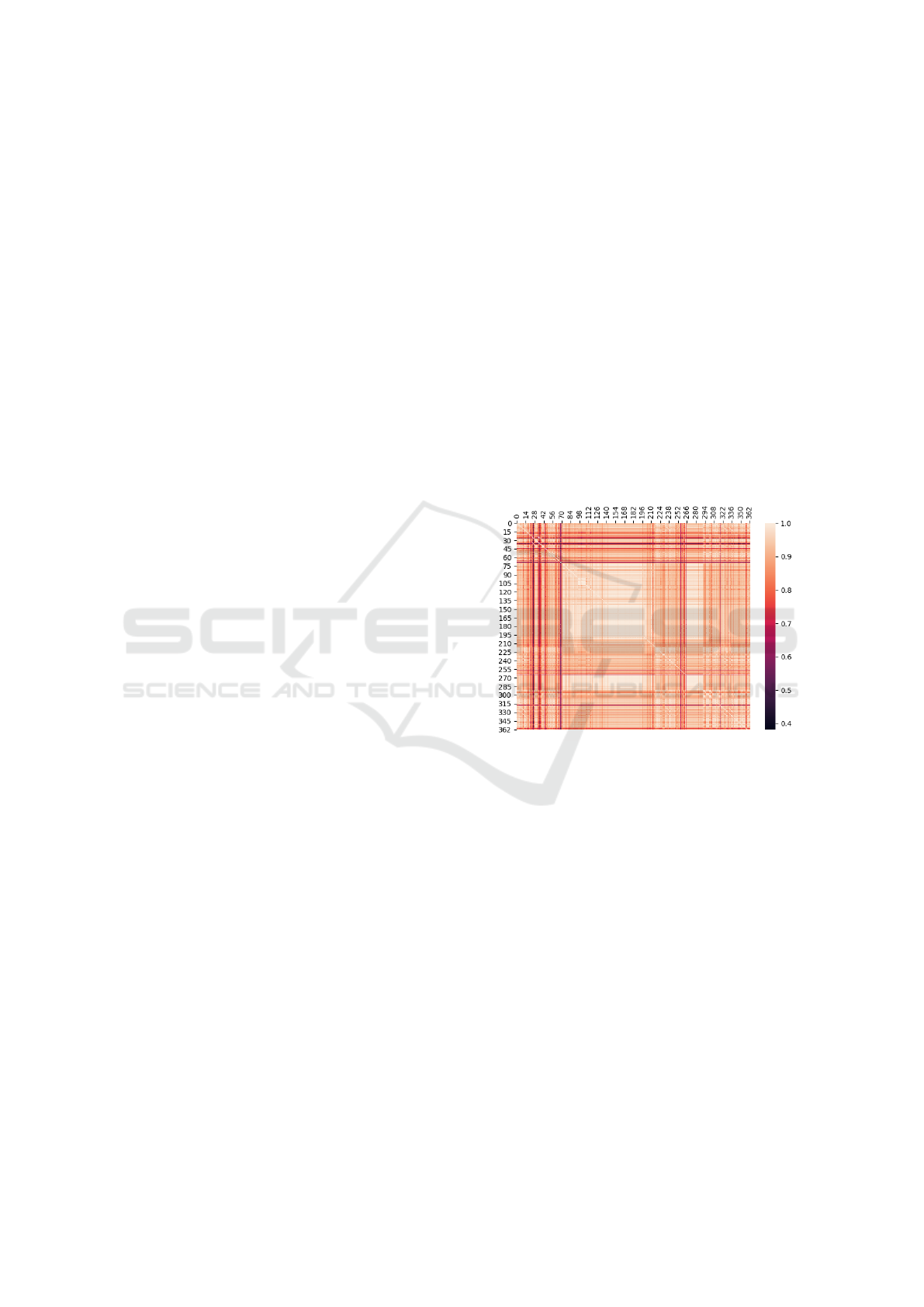
the same trend during learning. Figure 2 depicts a cor-

relation matrix for the 362 indicators, computed using

Spearman coefﬁcient (Mukaka, 2012). The darker a

point is, the least correlation between the correspond-

ing two indicators. Only a few of them are not much

correlated with the others (dark lines), and the major-

ity have a strong correlation (white areas). Indicators

with a perfect correlation to another one are deleted.

Figure 2: Correlation matrix between 362×362 indicators.

A third idea is to select the most relevant indica-

tors (for each variable) using feature importance tech-

niques (Guyon and Elisseeff, 2003). Algorithm 1 il-

lustrates this process by generating ranked lists of fea-

tures (lines 3 and 4) based on algorithms Extra Trees

(ET) and Random Forest (RF). The output of these

algorithms are merged, and to avoid strong impact of

a category of indicators (e.g., related to population),

an indicator is removed if its parent is already in the

list (lines 6 to 11). In the end, we obtain several list

of features noted L

which contain the most k relevant

indicators for variable v. We have chosen to retain

several lists containing from 10 to 100 indicators due

to the complexity of prediction.

When features have been selected, the learning

process can be run, as shown in the next section.

DATA 2020 - 9th International Conference on Data Science, Technology and Applications

298

Algorithm 1: Selection of relevant features.

input : set of indicators I , set of variables V

output: lists of features L

1 for v ∈ V do

2 L

←−

3 F

←− ET.rank_features(I );

4 F

←− RF.rank_features(I );

5 F ←− F

∪ F

;

/* sort, specific to general */

6 F ←− sort(F);

7 for f ∈ F do

8 p

←− parent(f);

9 if p

∈ F then

10 p

.score ←− p

.score+ f .score;

11 F ←− F − { f };

12 for k ∈ [10, 20, 30, 40, 50, 75, 100] do

13 L

←− top-K(F, k);

5 EXPERIMENTS

This section covers our preliminary experiments.

5.1 Experiment Protocol

We use the popular scikit-learn library for machine

learning (Pedregosa et al., 2011). We are in a classi-

ﬁcation problem and ﬁve scikit-learn algorithms have

been used

: Logistic Regression (LR), Random For-

est (RF), K-Nearest Neighbours (KNN), Support Vec-

tor Classiﬁcation (SVC), and AdaBoost (AB). Many

parameters have an impact in machine learning (Jor-

dan and Mitchell, 2015), and we tested several con-

ﬁgurations (e.g., weights, maximum depth in trees,

number of neighbours, distance metric) to retain the

best one. The annotated neighbourhoods are split

into 80% training data and 20% evaluation data with

cross-validation, as recommended in the literature

(Bruce and Bruce, 2017). We use accuracy as qual-

ity metric, i.e. the fraction of correct predictions. It

is common to have outliers in data, especially when

working with real-world data. They can be detected

using Isolation Forest algorithm for example, but it

requires a manual approbation (i.e., verifying that the

distribution conﬁrms the outlier). Although outliers

may decrease accuracy, we have a tiny supervised

dataset and removing outliers means even less super-

vised data in our context.

Other algorithms such as Stochastic Gradient Descent

or Nearest Centroid have been tested, but they mostly follow

the same trend or achieve insufﬁcient accuracy.

5.2 Results

The main objective is to correctly predict the values

for each environment variable of an IRIS. Recall that

we have generated, for each variable, lists of top-10,

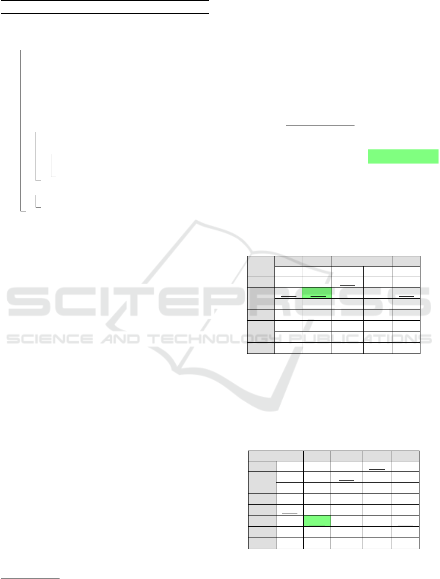
up to top-100 features. Tables 2 to 7 provides the

accuracy score (percentage) computed for each vari-

able using different algorithms. In these tables, the

baseline list I stands for all indicators (i.e., no fea-

ture selection) while L

represents a list of k selected

features. The underlined scores indicates the best re-

sult for an algorithm (i.e., by column). A bold score

means that the corresponding list of features achieves

a better score than the list I . The highlighted cells

correspond to the best score in the whole table.

Table 2 presents the quality results for the build-

ing type variable. Without feature selection, quality

spans from 36% to 57%. Smaller lists enable an im-

provement over list I (e.g., L

). The best score is

achieved by RF with list L

Table 2: Prediction quality for variable building type.

LR RF KNN SVC AB

I 46.6 57.0 55.2 45.5 36.5

44.3 59.3 57.8 44.7 41.7

49.2 60.0 56.3 43.6 43.6

45.1 58.9 55.9 43.6 32.1

46.2 59.3 54.8 43.2 27.6

46.6 58.9 54.8 45.5 32.4

44.3 58.2 55.2 45.9 32.0

100

43.6 57.0 55.2 45.5 36.5

Table 3 shows prediction quality for the usage

variable. The scores without selection is tighter, be-

tween 50% and 65%. A few of the smallest lists per-

form better than the baseline one, but without signiﬁ-

cant improvement. RF obtains the best result with list

Table 3: Prediction quality for variable usage.

LR RF KNN SVC AB

I 52.9 64.5 59.3 51.1 55.6

52.6 61.2 63.8 49.6 59.6

55.9 64.1 63.0 49.6 56.6

51.1 61.2 62.3 49.6 60.8

57.8 63.0 60.8 49.2 56.3

56.3 64.9 62.2 46.6 61.1

50.7 63.4 60.8 51.1 58.2

100

53.7 64.5 59.3 51.1 55.6

Table 4 provides accuracy scores for the land-

scape variable. Similarly to previous results, small

lists are able to improve quality over list I with three

algorithms. SVC obtains the same score whatever the

list.

Predicting the Environment of a Neighborhood: A Use Case for France

299

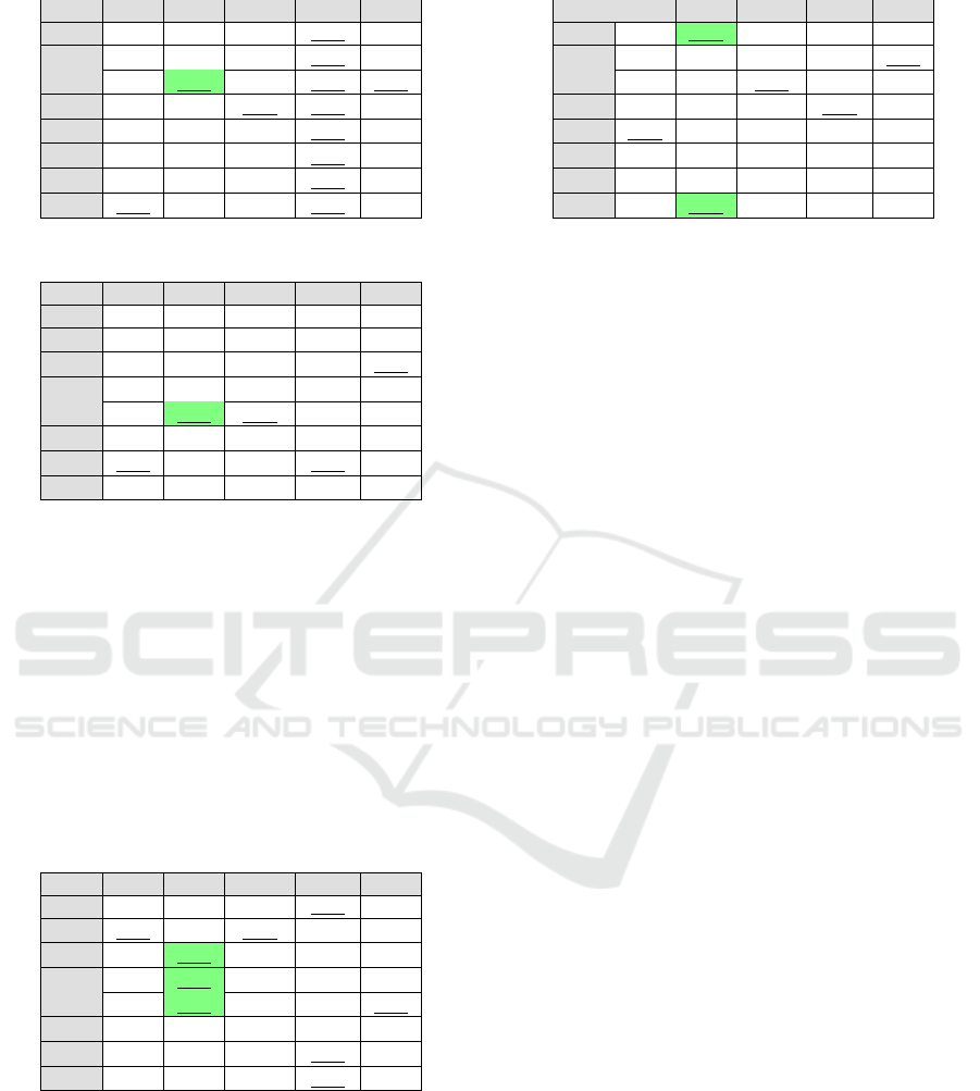
Table 4: Prediction quality for variable landscape.

LR RF KNN SVC AB

I 53.7 60.8 59.6 47.7 50.3

48.1 62.7 59.6 47.7 51.8

51.5 63.0 60.4 47.7 52.6

50.3 60.8 61.9 47.7 52.5

49.2 62.7 61.5 47.7 49.2

47.7 61.5 61.1 47.7 48.1

52.6 62.3 59.3 47.7 48.5

100

56.3 60.8 59.6 47.7 50.3

Table 5: Prediction quality for variable social class.

LR RF KNN SVC AB

I 44.4 51.1 42.1 45.5 36.5

43.6 46.6 43.9 44.7 41.7

39.1 46.6 45.1 43.6 43.6

41.4 49.6 45.1 43.6 32.1

39.1 51.8 46.6 43.2 27.6

42.1 48.1 44.3 45.5 32.4

45.1 48.1 44.0 45.9 32.0

100

40.7 51.1 42.1 45.5 36.5

Table 5 depicts quality results for the social class

variable. The lists of selected features, either small

or large depending on the algorithm, allows a better

quality in a few cases. The best score is slightly above

50%, which shows that this variable is difﬁcult to pre-

dict. Yet, many features describe incomes (median,

per decile), population characteristics (number of stu-

dents, employees, farmers, unemployed, etc.).

Table 6 details quality obtained for the morpho-

logical position. The L

list mainly wins against the

baseline list, except with SVC which achieves similar

scores (44%) whatever the features.

Table 6: Prediction quality for variable morphological.

LR RF KNN SVC AB

I 46.6 59.7 58.2 44.7 45.8

48.5 60.0 60.8 44.0 49.9

44.0 61.2 58.5 44.4 48.5

39.2 61.2 58.2 44.4 48.8

33.5 61.2 58.6 44.4 50.7

36.1 59.3 57.4 44.4 46.2

41.3 60.8 57.1 44.7 49.2

100

43.2 59.7 58.2 44.7 45.8

Table 7 is dedicated to geographical position.

Scores are far lower than for other variables (33% as

best value), which is not surprising given the a-priori

irrelevant indicators for this prediction. Still, small

lists mostly perform better than the baseline.

We conclude this experimental section with a

discussion. Best scores range from 33% for geo-

graphical position and 50% for social class to 60-

65% for the remaining four variables. Although al-

Table 7: Prediction quality for variable geographical.

LR RF KNN SVC AB

I 22.0 33.6 27.2 25.0 15.6

25.3 29.9 27.6 24.6 21.9

26.1 31.3 29.5 25.3 20.1

26.1 31.7 28.3 27.2 17.5

29.1 32.8 28.3 24.6 17.1

25.0 32.1 27.2 23.8 19.0

24.6 32.8 27.2 25.0 17.9

100

24.6 33.6 27.2 25.0 15.6

gorithms obtain different scores with the baseline list,

their results mainly improve by a few percent (in av-

erage per column) when using other lists of features,

which could demonstrate that current indicators are

not sufﬁcient or useful. These results are promising,

but still require improvements, especially regarding

the representativeness issues presented in Section 4.1.

It was not possible to predict on a sufﬁcient num-

ber of new IRIS because the manual veriﬁcation is

time-consuming, as explained in Section 3.1. Among

the ten algorithms and conﬁgurations we have tested

so far, Random Forest seems to be the most interest-

ing in our context because it achieves all best scores.

Some algorithms were not suitable, for instance SVC

requires many features (best results with all indicators

or with largest lists of features). Our algorithm for

feature selection has also proven useful, since many

lists outperform the baseline (whatever the algorithm

or variable). Lists of 20 up to 50 features are particu-

larly effective. However, the improvement is not sig-

niﬁcant (a few percent at best compared to baseline).

On the contrary, larger lists (top-100) usually provide

the same quality as the baseline.

6 CONCLUSION

In this paper, we have presented a use case for pre-

dicting the environment of any neighbourhood in

France through six descriptive variables. We have

studied the representativeness of our 270 annotated

neighbourhoods compared to the whole set of 49,800

to detect some bias. Due to a large quantity of avail-

able indicators, we also selected a subset for each

variable. Our experiments show that (small) lists gen-

erated with our feature selection perform better than

a learning using all indicators. However, the overall

prediction scores need to be improved before predict-

ing at a larger scale.

The main perspective is to achieve better predic-

tion results. Our ﬁrst results could be exploited by so-

cial science researchers in order to facilitate the man-

ual annotation of neighbourhoods, thus increasing the

amount of examples. Another possibility could be the

DATA 2020 - 9th International Conference on Data Science, Technology and Applications

300

generation of a bigger synthetic dataset, which share

similarities with the 49,800 neighbourhoods. We also

plan to integrate prices and points of interest (that

could reﬂect the nature of a neighbourhood, for in-

stance an organic shop is usually found in middle or

upper class neighbourhoods).A fourth perspective is

the correlation between variables, which are not to-

tally independent. For instance, a rural area has more

chances to be classiﬁed as countryside and to host

houses. The prediction of a given variable could im-

pact the classiﬁcation of others, especially the most

difﬁcult ones such as geographical or social. Finally,

we plan to release a tool named predihood for letting

researchers implement and test their classiﬁcation al-

gorithms on our dataset.

ACKNOWLEDGEMENTS

This work has been partially funded by LABEX

IMU (ANR-10-LABX-0088) from Université de

Lyon, in the context of the program "Investissements

d’Avenir" (ANR-11-IDEX-0007) from the French

Research Agency (ANR), during the HiL project

REFERENCES

Barret, N., Duchateau, F., Favetta, F., Miquel, M., Gen-

til, A., and Bonneval, L. (2019). À la recherche du

quartier idéal. In EGC, page 429–432.

Bellahsène, Z., Bonifati, A., and Rahm, E. (2011). Schema

matching and mapping. Springer.

Bigot, R., Croutte, P., Müller, J., and Osier, G. (2011). Les

classes moyennes en europe. Le CRÉDOC, Cahier de

recherche, 282.

Bonneval, L., Duchateau, F., Favetta, F., Gentil, A., Jelassi,

M. N., Miquel, M., and Moncla, L. (2019). Étude des

quartiers : déﬁs et pistes de recherche. In EGC.

Bruce, P. and Bruce, A. (2017). Practical Statistics for Data

Scientists: 50 Essential Concepts. O’Reilly.

Caragliu, A., Del Bo, C., and Nijkamp, P. (2011). Smart

cities in europe. J. of urban technology, 18(2):65–82.

Christen, P. (2012). Data matching: concepts and tech-

niques for record linkage, entity resolution, and dupli-

cate detection. Springer Science & Business Media.

Cranshaw, J., Schwartz, R., Hong, J., and Sadeh, N. (2012).

The livehoods project: Utilizing social media to un-

derstand the dynamics of a city. In AAAI Conference

on Weblogs and Social Media.

Delmelle, E. C. (2015). Five decades of neighborhood clas-

siﬁcations and their transitions: A comparison of four

us cities, 1970–2010. Applied Geography, 57:1 – 11.

http://imu.universite-lyon.fr/projet/hil/

Dhar, V. (2013). Data science and prediction. Communica-

tions of the ACM, 56(12):64–73.

Donoho, D. (2017). 50 years of data science. J. of Compu-

tational and Graphical Statistics, 26(4):745–766.

Guyon, I. and Elisseeff, A. (2003). An introduction to vari-

able and feature selection. J. of Machine Learning

Research, 3(3):1157–1182.

Halevy, A., Rajaraman, A., and Ordille, J. (2006). Data

integration: the teenage years. In VLDB, pages 9–16.

Jordan, M. I. and Mitchell, T. M. (2015). Machine learn-

ing: Trends, perspectives, and prospects. Science,

349(6245):255–260.

Le Falher, G., Gionis, A., and Mathioudakis, M. (2015).

Where Is the Soho of Rome? Measures and Algo-

rithms for Finding Similar Neighborhoods in Cities.

ICWSM, 2:3–2.

Lillesand, T., Kiefer, R. W., and Chipman, J. (2015). Re-

mote sensing and image interpretation. Wiley & Sons.

Mukaka, M. M. (2012). A guide to appropriate use of corre-

lation coefﬁcient in medical research. Malawi medical

journal, 24(3):69–71.

Ojo, A., Curry, E., and Zeleti, F. A. (2015). A tale of open

data innovations in ﬁve smart cities. In Int. Conf. on

System Sciences, pages 2326–2335. IEEE.

Pedregosa, F., Varoquaux, G., Gramfort, A., Michel, V.,

Thirion, B., Grisel, O., Blondel, M., Prettenhofer, P.,

Weiss, R., Dubourg, V., Vanderplas, J., Passos, A.,

Cournapeau, D., Brucher, M., Perrot, M., and Duch-

esnay, E. (2011). Scikit-learn: Machine learning in

Python. J. of Machine Learning Research, 12:2825–

2830.

Shen, W., Wang, J., and Han, J. (2015). Entity linking with

a knowledge base: Issues, techniques, and solutions.

TKDE, 27(2):443–460.

Tang, E. and Sangani, K. (2015). Neighborhood and price

prediction for san francisco airbnb listings.

Yu, M., Li, G., Deng, D., and Feng, J. (2016). String simi-

larity search and join: a survey. Frontiers of Computer

Science, 10(3):399–417.

Yuan, X., Lee, J.-H., Kim, S.-J., and Kim, Y.-H. (2013). To-

ward a user-oriented recommendation system for real

estate websites. Information Systems, 38(2):231–243.

Zhang, A. X., Noulas, A., Scellato, S., and Mascolo, C.

(2013). Hoodsquare: Modeling and recommending

neighborhoods in location-based social networks. In

Social Computing, pages 69–74. IEEE.

Predicting the Environment of a Neighborhood: A Use Case for France

301