
Evaluation of Alternative Propulsion Concepts for Mobile Machinery:
A Modelling Approach using the Example on LNG-powered Port
Handling Equipment
Patrick Driesch, Kai Horwat, Niko Maas and Dieter Schramm
Chair of Mechatronics, University of Duisburg-Essen, Lotharstraße 1, 47057 Duisburg, Germany
Keywords:
Semi-physical Modelling, Evaluation of Alternative Propulsion Concepts.
Abstract:
The prevailing climate goals and related emission limits for fleets are forcing industry to consider alternative
fuels alongside established fuels such as diesel and gasoline. A conversion of a fleet of vehicles to another
source of power comes along with an investment of money and a risk that the day-to-day operations of the
new drive technology do not provide the expected effects regarding the fuel consumption and the exhaust
gas emissions. In order to assess these barriers in advance, this paper presents an approach of a simulation
tool based on a semi-physical modelling of the powertrain of mobile machinery to predict the impact of a
conversion of a fleet from diesel to liquefied natural gas (LNG) in case of fuel consumption and exhaust gas
emissions. For the semi-physical model, a combination of a physical model of the vehicle and powertrain
dynamics and a black box modelling of the internal combustion engine by artificial neural networks is chosen.
The simulation tool will be used in the future to assess the feasibility of converting the drive system from port
transhipment facilities to LNG. The work was carried out as part of the research project LeanDeR financed by
the European Regional Development Fund (ERDF).
1 INTRODUCTION
The climate targets of the European Union pose ma-
jor challenges for the development and the use of
vehicles. By the year 2030 greenhouse gas emis-
sions have to be reduced by 40 % compared to the
level of 1990 and by 2050 climate neutrality is to
be achieved, (European Commission, 2018). In ad-
dition to the reduction of greenhouse gas emissions,
it is also necessary to reduce the emission of air pol-
lutants. Beside the industry and energy sector, the
traffic and transport sector is a significant producer of
emissions, (International Energy Agency, 2019). In
Germany, e. g., the traffic and transport sector emit-
ted about 18.4 % of the energy-related greenhouse
gas emissions in 2017, (Federal Ministry for the En-
vironment, Nature Conservation and Nuclear Safety,
2019). The term transport is often confined to the cat-
egory of road vehicles, as these are used in the imme-
diate vicinity of the population and their living envi-
ronment and can therefore be directly observed. An-
other segment of vehicles that differs in this respect
is the so-called mobile machinery. Unlike road vehi-
cles, which are primarily used to transport goods from
one place to another, these machinery have the task
to perform mechanical work in addition to the trans-
port task, (Geimer and Pohlandt, 2014). A study by
(Helms et al., 2017) shows that these machinery emit
a non-negligible proportion of greenhouse gas emis-
sions and air pollutants. Achieving the mentioned
goals will require a conversion from established fossil
fuels towards alternatives which provide less exhaust
gas emissions. Suitable alternatives are, e. g., natural
gas or an electrification or hybridisation of the pow-
ertrain, (Milojevi
´
c et al., 2018; Lajunen et al., 2018).
All these energy sources have in common, that there
is a lack of sufficient tank or charging infrastructure
to enable a changeover at short notice. In addition,
due to the fact that most of the mobile machinery is
diesel-driven and many different types of vehicles are
included in this section, there is an insufficient re-
search on whether and how everyday operation with
alternative fuels can be performed. In order to coun-
teract this, the operation of a multimodal liquefied
natural gas (LNG) station infrastructure is tested in
the port of Duisburg, called duisport, as part of the
research project LeanDeR. To investigate the suitabil-
ity of LNG for everyday use, two mobile machinery
from the entire duisport fleet were tested with natural
gas and compared with a similar diesel-powered ve-
Driesch, P., Horwat, K., Maas, N. and Schramm, D.
Evaluation of Alternative Propulsion Concepts for Mobile Machinery: A Modelling Approach using the Example on LNG-powered Port Handling Equipment.
DOI: 10.5220/0009872502250232
In Proceedings of the 10th International Conference on Simulation and Modeling Methodologies, Technologies and Applications (SIMULTECH 2020), pages 225-232
ISBN: 978-989-758-444-2
Copyright
c
2020 by SCITEPRESS – Science and Technology Publications, Lda. All rights reserved
225

hicle. For this purpose, measurement data from the
LNG and the diesel-driven vehicles were recorded by
autonomous data-logging systems whilst their every-
day operation. One of these vehicles, a terminal trac-
tor (see figure 1), is used to manoeuvre trailers around
the port area. The terminal tractor considered in the
course of the research project is powered by LNG in
a mono-fuel operation.
Figure 1: Diesel- and LNG-driven terminal tractors at the
duisport, (Duisburger Hafen AG, 2019).
Since the operation of a LNG filling station be-
yond the end of the project at the end of May 2020,
only for the refueling of two vehicles, appears uneco-
nomical, it must be examined whether a fleet-wide
switch from diesel to natural gas would bring both
economic and ecological advantages. Because a fail-
ure of the machinery directly extends to further pro-
cess steps in the form of process follow-up costs, a so-
lution is needed to weigh up a fleet-wide changeover
with low risk and economic expenditure simultane-
ously. In the course of this paper, a simulation tool
will be presented using the example of the terminal
tractors. This tool enables the upscaling for a com-
plete changeover of a fleet of mobile machinery to
an alternative fuel. Based on the detailed database
of the individual measured vehicles, semi-physical
models of the vehicles' powertrains need to be devel-
oped. These models shall predict the fuel consump-
tion and exhaust gas emissions of the other vehicles
of the entire fleet in the respective powertrain. For
the rest of the fleet only the knowledge of the vehicle
speed, its payload and the current ambient tempera-
ture is required. The vehicle speed can be recorded
during daily operation without a great effort. To es-
timate the payload of the port handling equipment,
an analysis of the performed manoeuvring orders can
be achieved from the terminal operating system. In-
formation about the ambient conditions can be taken
from accessible weather databases. By a fusion of
these information depending on the respective time
stamp the required model input is provided.
In section 2 the methodical approach to the de-
velopment of the simulation tool is described. After-
wards the modelling is explained in section 3. Finally,
section 4 provides a summary and outlook for future
work.
2 METHODICAL APPROACH
The objective of a simulation environment for predict-
ing a fleet-wide changeover from diesel-driven termi-
nal tractors to natural gas propulsion as described in
section 1 requires a systematic approach. For this pur-
pose, the following steps based on (Verein Deutscher
Ingenieure e.V., 2016) are fulfilled:
1. Formulation of tasks and objectives
2. Structural and functional analysis
3. Data collection and analysis
4. Determination of the relevant model aspects
5. Problem decomposition
6. Determination of the model type
7. System and process description
2.1 Formulation of Tasks and
Objectives
The goal of the simulation tool is to estimate unknown
process variables of the remaining fleet vehicles in
everyday operation with conventional and alternative
fuels. For this purpose, the operation of the vehicles
must be simulated with one diesel and one natural gas
powertrain each, so that the resulting fuel consump-
tion and exhaust gas emissions for both drive types
can be concluded. Afterwards the sum of the fuel con-
sumption and exhaust gas emissions of the whole fleet
have to be calculated.
2.2 Structural and Functional Analysis
The total fuel consumption m
F, p
of the vehicle fleet
for p different powertrains as well as the correspond-
ing masses of exhaust gas emissions m
E
α
, p
of chemi-
cal compounds α like CO
2
occur as unknown process
variables and thus as output variables of the simula-
tion tool. As mentioned before, the velocity v and
the payload m
Trailer
of the terminal tractors as well as
the current ambient temperature T
Amb
during every-
day operation are used as input variables. These daily
operations can be subdivided into several rides from
one shutdown of the engine to the next. Each ride
consists of a time-dependent vector of inputs, so that
for an assumed fleet of n vehicles with m rides each
∑
n
i=1
m(i) time-dependent input vectors are available.
Thus, for an estimation of the fuel consumption and
SIMULTECH 2020 - 10th International Conference on Simulation and Modeling Methodologies, Technologies and Applications
226

exhaust gas emissions of a whole fleet, the simulation
process has the structure illustrated in figure 2.
Every ride needs to be simulated with p different
powertrains. Therefore a simulation framework pre-
dicts the mass flow of the fuel ˙m
F, p
and the mass flows
˙m
E
α
, p
of the corresponding exhaust gas emissions of
chemical compounds α for every ride with p power-
trains.
Ride
of rides
of Veh
i
j
m
v
i,j
m
Trailer,i,j
Simulation
tool with
powertrains
p
Fleet of
vehiclesn
Veh
i
while ≤j m
while ≤i n
m
E ,p, ,ji
α
m
F,p,i,j
n
∑
i=1
∑
j=1
m
. .
∫ td
m
E ,p,i,j
α
m
F,p,i,j
m
E ,p
α
m
F,p
Postprocessing
T
Amb,i,j
Figure 2: Structure of the simulation process.
In total p ·
∑
n
i=1
m(i) simulations must be carried
out. To estimate the total mass of fuel and exhaust
gas emissions for the whole fleet for p powertrains,
the mass flows are integrated and added up for every
powertrain in a postprocessing.
2.3 Data Collection and Analysis
The development of simulation models requires
knowledge about the system which shall be described.
This is gained from the analysis of the everyday
operation of the reference vehicles during a mea-
surement period from January 2019 to May 2020 in
course of the research project LeanDeR. The vehi-
cles were equipped with self-sufficient data-logging
systems which permanently recorded measurements
of the ambient temperature, the GPS data set, the ac-
celerations in three space dimensions as well as data
from the CAN bus of the vehicles with a measure-
ment frequency of 1 Hz. Thus measurements like the
engine speed, its torque, the temperature of the en-
gine coolant, the massflow of exhaust gas recircula-
tion, the massflow of intake air and the massflow of
consumed fuel were available. Furthermore, the vol-
ume concentration of the chemical compounds CO,
CO
2
, NO
x
, CH
4
and SO
2
of the exhaust gas emissions
were measured at the exhaust pipe with an exhaust
gas emissions measurement system of type J2KNpro
from the manufacturer ecom. Since permanent opera-
tion of the exhaust gas analysis device is not possible
due to protective mechanisms in the device against the
poisoning of individual sensors and a renewed cali-
bration of the sensors to prevent measurement drift,
measurements were performed at specified times. To
determine the mass flows of the respective exhaust
gas component, a mass-based calculation according
to (European Parliament and the Council, 2017) was
carried out. At the end of February 2020 the data base
consisted of 11,460 km driving distance and 1,244 h
driving duration of the diesel-driven terminal trac-
tor. For the LNG-driven terminal tractor 11,909 km
driving distance and 1,237 h driving duration were
recorded. A distance of 261.3 km at a driving dura-
tion of 27.3 h were driven by the LNG-driven termi-
nal tractor while an exhaust gas emissions measure-
ment was executed. For the diesel-driven terminal
tractor 138.9 km driving distance at 14.1 h of driv-
ing time during exhaust gas emissions measurement
were recorded. In addition to the measurements of
the motion of the vehicles, information regarding the
load of the vehicles at specific timeslots can be taken
by the terminal operating system. This system orga-
nizes the cargo handling and provide the gross weight
of handled container which are placed on the trail-
ers. These gross weight of the container includes the
weight of the container itself and the goods inside the
container, (Zhao et al., 2020).
2.4 Determination of the Relevant
Model Aspects
Internal variables are required to implement the rela-
tionship between the input and output vectors shown
in the system structure in figure 2. An analysis of the
physical relationship between the inputs and outputs
points out, that the combustion engine of the vehicles
acts as the essential interface. It converts the chem-
ical energy of the fuel by internal combustion into
mechanical power on the crankshaft, causing exhaust
gas emissions. This mechanical power is transferred
through the powertrain to provide the required driving
force at the wheels. Accordingly, the engine speed
n
Engine
and its torque M
Engine
are defined as internal
variables of the simulation tool.
2.5 Problem Decomposition
By considering vectors of internal variables, a defined
connection exists between the input and output vec-
tors of the simulation tool. Thus the overall simula-
tion model can be subdivided into two subsystems for
every powertrain p, as figure 3 illustrates, where the
internal variables are the output of the first and the in-
put for the second subsystem. Thus both subsystems
can be developed in parallel and optimized specifi-
cally with the available database. The first subsystem
includes the modelling of the dynamics of the vehicles
Evaluation of Alternative Propulsion Concepts for Mobile Machinery: A Modelling Approach using the Example on LNG-powered Port
Handling Equipment
227

and their powertrains to determine n
Engine
and M
Engine
by v, T
Amb
and m
Trailer
. To estimate the mass flows
of the fuel consumption ˙m
F
and the chemical com-
pounds of the exhaust gas emissions ˙m
E
α
, the second
subsystem represents a model to describe the com-
bustion process of the engine of the respective pow-
ertrain. This model uses the outputs of the first sub-
system and also some of the global inputs, e. g., the
ambient temperature T
Amb
as inputs.
Figure 3: Problem decomposition into two subsystems for
every powertrain.
2.6 Determination of the Model Type
The subsystems can be developed with different mod-
elling methods. According to (Schramm et al., 2018),
the dynamic behaviour of real processes is carried out
either by theoretical modelling based on physical laws
or by experimental modelling based on measurements
of inputs and outputs. A modelling by physical laws
grants the advantages that the results of the simulation
are easier to interpretate physically, (Dubois, 2018).
Thus a better understanding of the model is given
but unknown physical parameters have to be identi-
fied. Experimental modelling, also called black-box
modelling, based on a mathematical description of the
relationship between the input and output measure-
ments by, e. g., an artificial neural network (ANN) al-
lows modelling of the system without sound process
knowledge, (Xu, 1997).
For the development of the simulation tool a semi-
physical modelling, i. e. a combination of both mod-
elling forms, is chosen. Because some physical pa-
rameters of the vehicles' mechanical powertrain are
provided by the manufacturer, for the first subsys-
tem a physical modelling approach is applied. Since
many different drivers with a variety of driving styles
are working with the terminal tractors, a backward-
facing quasi-stationary model of the vehicles' longi-
tudinal dynamics and powertrain is used. This type
of model does not require a driver model and the nec-
essary torque and speed of the engine is calculated
backwards through the powertrain based on the power
requirement at the wheels to overcome the driving re-
sistances, (Mohan et al., 2013; Wipke et al., 1999).
The mathematical modelling of internal com-
bustion engines is complex and requires knowledge
about thermodynamic conditions, e. g., in the com-
bustion chamber and intake as well as exhaust man-
ifolds, (Schramm et al., 2020; Guzzella and Onder,
2010; Serikov, 2010). Due to the fact that no mea-
surements of thermodynamic conditions of the com-
bustion engine were available, a black-box modelling
approach like in (Serikov, 2010) is used. The estima-
tion of the mass flow of fuel ˙m
F
and corresponding
mass flows of the chemical compounds ˙m
E
α
of the
exhaust gas emissions shall be done by ANNs using,
e. g., n
Engine
and M
Engine
as inputs.
2.7 System and Process Description
The system and process description represents the de-
velopment of the system structure shown in figure 2
and the subsystems illustrated in figure 3 for p power-
trains. Since working with ANNs with frameworks
like Tensorflow in the high level programming lan-
guage Python is very common, the implementation of
the physical models as well as the development of the
ANNs is performed in Python. This means that both
subsystems can be connected in the same software en-
vironment. In the following section 3 the modelling
of both subsystems is described in detail.
3 MODELLING OF THE
SUBSYSTEMS
The simulation tool consists of two subsystems which
are based on different modelling approaches. After-
wards both subsystems are explained. In section 3.1
the physical modelling of the vehicle and powertrain
dynamics is shown. The black-box modelling of the
combustion engine is presented in 3.2.
3.1 Modelling of the Vehicle Dynamics
As mentioned before, a backward directed model of
the vehicles' longitudinal dynamics and its power-
train shall be applied to estimate the engine speed
and the torque from the vehicle's velocity, its payload
and the ambient temperature. First, based on a time-
dependent input vector
x(t) =
v(t) T
Amb
(t) m
Trailer
(t)
(1)
as well as vehicle and environmental parameters
like the vehicle mass m
V
, its front cross-sectional
SIMULTECH 2020 - 10th International Conference on Simulation and Modeling Methodologies, Technologies and Applications
228

area A
V
, its drag coefficient c
W
, the air density ρ,
the acceleration due to gravity g and the dynamic
rolling radius of the wheels r
dyn
, the acting driving
resistances are determined according to (Schramm
et al., 2020). It is assumed that the vehicle is driving
straight forward and the wheels roll slip-free. Since
the vehicles are moved on a surface without any
significant gradient, the road inclination and thus
the slope resistance is ignored. Also not considered
is the wind speed, which is more or less evenly
distributed in the spatial directions over time. In total,
the acceleration resistance F
Acc
, the wind resistance
F
Air
, the rolling resistance F
Roll
and the resistance
by pulling the trailer F
Trailer
counteract the vehicle's
movement as shown in figure 4.
F
Air
v
F
Acc
F
Roll,F
F
Roll,R
F
Trailer
F
Drive
Figure 4: Acting driving resistances upon the terminal trac-
tor in longitudinal direction, (Terberg Benschop, 2015).
The required drive force F
Drive
sums up the driv-
ing resistances. Thus, the corresponding drive power
P
Drive
can be calculated by equation (2).
P
Drive
= F
Drive
· v
= (F
Acc
+ F
Air
+ F
Roll
+ F
Trailer
) · v
(2)
The acceleration resistance F
Acc
describes the
translational and rotational inertia of the vehicles
which counteracts the change in motion and can be
determined by equation (3).
F
Acc
= m
V
· (1 + λ ) ·
dv
dt
(3)
Here λ represents the rotational mass surcharge
factor, which expresses the rotational inertia J
PT
in the
powertrain in the form of a translatory force according
equation (4).
λ =
J
PT
(m
V
· r
2
dyn
)
(4)
The air resistance F
Air
represents the aerodynamic
resistance of the vehicle and is considered with equa-
tion (5).
F
Air
=
1
2
· c
W
· A
V
· ρ · v
2
(5)
According to (Mitschke and Wallentowitz, 2014)
the wheel resistance results mainly from the rolling
resistance F
Roll
. Taking into account, that the wheels
of the front and rear axis are similar, the rolling resis-
tance can be described by equation (6) with a rolling
resistance coefficient f
R,V
.
F
Roll
= f
R,V
· m
V
· g (6)
The pulling resistance required to move a trailer
is considered by a separate modelling of the
trailer, (Haken, 2015). The rotational inertia of the
trailers' wheels and the trailers' air resistance can be
assumed to be negligible compared to the transla-
tional inertia of the trailers' mass and rolling resis-
tance of its wheels. Thus the total resistance by
pulling the trailers can be described by equation (7)
with a rolling resistance coefficient f
R,Trailer
.
F
Trailer
= f
R,Trailer
· m
Trailer
· g + m
Trailer
·
dv
dt
(7)
In order to determine n
Engine
and M
Engine
, a mod-
elling of the vehicles' powertrains as shown in figure
5 is carried out. The powertrains include the combus-
tion engine, an automatic transmission with a torque
converter and an axle drive. Besides the mechanical
power to drive the vehicle, auxiliaries, e.g., the alter-
nator and the air conditioning are also driven.
Engine
Torque
Converter
Automatic
Transmission
Auxiliaries
Axle
Drive
v
P
Drive
⁄
2
P
Drive
⁄
2
P
AD
P
AT
P
TC
P
AUX
Figure 5: Overview of the terminal tractors' powertrains.
The drive power P
Drive
is used as the input of the
powertrain model to estimate the engine speed and the
torque backwards through the entire powertrain. Be-
ginning with equations (8) and (9) the speed and the
torque of the tires, which equals the output speed and
the torque of the axle drive, is calculated.
n
Tires
=
v
2 · π · r
dyn
(8)
M
Tires
=
P
Drive
2 · π · n
Tires
(9)
By taking into account the gear ratio i
AD
and ef-
ficiency η
AD
of the axle drive, its associated input
speed and torque can be determined by the equations
(10) and (11). Those values equal the output speed
and the torque of the automatic transmission.
Evaluation of Alternative Propulsion Concepts for Mobile Machinery: A Modelling Approach using the Example on LNG-powered Port
Handling Equipment
229

n
AD
= n
Tires
· i
AD
(10)
M
AD
=
M
Tires
i
AD
· η
AD
(11)
The input of the automatic transmission is calcu-
lated with a gear ratio i
AT
which depends on the se-
lected gear G
AT
and an efficiency η
AT
by equations
(12) and (13).
n
AT
= n
AD
· i
AT
(G
AT
) (12)
M
AT
=
M
AD
i
AT
(G
AT
) · η
AT
(13)
Due to the fact that the selected gear is not in-
cluded in the input vector x(t), an ANN as shown in
figure 6 shall be used to predict the selected gear G
AT
.
According to (Jeoung et al., 2020) the shifting of gear
in automatic transmissions is controlled by the veloc-
ity of the vehicle and the position of the accelerator
pedal. A change of the accelerator pedal position is
related to a change of torque and thereby to a change
of vehicles velocity and thus its acceleration. That is
why the vehicle speed v and acceleration
dv
dt
are used
as inputs, as figure 6 illustrates. The corresponding
gear ratio i
AT
(G
AT
) is selected from a lookup-table
filled with information from the data sheet of the man-
ufacturer.
v
G
AT
dv
dt
Figure 6: Neural network to predict the selected gear.
A torque converter is placed between the transmis-
sion and the engine to overcome speed differences
when starting from engine idling. Since sufficient
information about the dynamics of the torque con-
verter are not available, a quasi-stationary modelling
approach based on characteristic values from the data
sheet of the torque converter according to (Luz, 2015)
is used. The desired engine speed and the torque cor-
respond to the input speed n
TC
and the torque M
TC
of
the torque converter taking into account an efficiency
η
TC
as shown in equation (14) and (15).
In addition, the engine has to power auxiliaries,
which are considered by a sum of n different mechan-
ical loads M
AUX,n
by
∑
n
i=1
M
AUX,i
, (Schramm et al.,
2020).
n
Engine
= n
TC
(14)
M
Engine
=
M
TC
η
TC
+
n
∑
i=1
M
AUX,i
(15)
In order to decide, whether the air condition-
ing is heating or cooling, an ambient-temperature-
dependent energy demand shall be considered.
3.2 Modelling of the Combustion
Engine
The combustion process of the engines measured dur-
ing the research project is modelled as a black-box.
In general, the model has to reply two questions for
every time step based on knowledge from its inputs:
• Which mixture of fuel, air and recirculated ex-
haust gas was burned in the combustion chamber?
• Which type and amount of exhaust gas emissions
are generated?
It was found that multiple factors can influence the
fuel consumption, exhaust gas emissions and the
performance of the engine as, e. g., the temperature
of the ambient air, the engine coolant temperature
or the rate of exhaust gas being recirculated to the
combustion chamber, (Abdullah et al., 2015; Abdel-
ghaffar et al., 2002; Hussain et al., 2012). Therefore
all the above-mentioned variables are considered in
the black-box modelling of the combustion engine.
To answer both questions, the engine model is
divided into two ANNs, using the outputs of the first
one as input for the second ANN, as shown in figure 7.
Figure 7: Structure of the black-box engine model.
In the first ANN the calculated n
Engine
and M
Engine
and the measured T
Amb
are used as inputs. The fourth
input, the engine coolant temperature T
EC
, is neither
calculated nor measured during the operation of the
entire fleet. This measurement value is just known
from the individual vehicles, but because of its im-
portance regarding the engines performance it is also
considered as an input. It is therefore up to the user
to define these temperatures in order to study engine
SIMULTECH 2020 - 10th International Conference on Simulation and Modeling Methodologies, Technologies and Applications
230
performance under different engine conditions such
as cold start or engine warm-up. The outputs of the
first ANN – the mass flow of fuel ˙m
F
, the mass flow
of air ˙m
Air
and mass flow of recirculated exhaust gas
˙m
EGR
– answer the first question.
The second ANN aims to answer the second ques-
tion by estimating the mass flow of carbon diox-
ide ˙m
E,CO
2
, carbon monoxide ˙m
E,CO
, nitrogen oxides
˙m
E,NO
x
, methane ˙m
E,CH
4
and sulphur dioxide ˙m
E,SO
2
.
Therefore the inputs of the first ANN as well as its
outputs are used as inputs to the second ANN.
4 SUMMARY AND OUTLOOK
This paper introduces an approach for a simulation
tool with which a complete conversion of a fleet of
mobile machinery to an alternative fuel can be scaled
up using measurements of individual vehicles. The
simulation tool includes semi-physical models of p
different powertrains to estimate the fuel consump-
tion and exhaust emissions of the entire fleet for ev-
ery powertrain setup. In this paper the simulation tool
is explained using the example of terminal tractors
and both, a diesel- and LNG-driven powertrain. Each
semi-physical model consists of a combination of a
physical modelling of the driving and powertrain dy-
namics and a black-box modelling of the engine by ar-
tificial neural networks. The development and param-
eterization of the models is fulfilled by measurements
of the everyday operation of two reference vehicles.
As inputs for the simulation tool measurements of the
time-dependent velocity v, ambient temperature T
Amb
and payload m
Trailer
of the rides of the vehicles of a
fleet are necessary. Based on these information the
simulation tool predicts the massflows of fuel ˙m
F
and
of the corresponding exhaust gas emissions ˙m
E
α
for
every powertrain p during the ride. For the calcu-
lation of the total mass of fuel and emissions of the
entire fleet for p powertrains, in a postprocessing the
simulation results for every ride and every powertrain
p are integrated and added up.
At the time of writing this paper, the physical
models of the vehicle and powertrain dynamics are
implemented. The ANNs for the prediction of the
gear provide a sparse categorical accuracy of 95,4%
(LNG) and 96,4 % (Diesel). Unknown physical para-
meters like the rolling resistance coefficient f
R,V
were
estimated by measurements of planed test drives in
which the terminal tractors did not pull any trailer.
The evaluation of the calculated and measured n
Engine
and M
Engine
during the test drives resulted in a mean
absolute error of 25.3 rpm and 21.9 Nm for the LNG-
and 30 rpm and 24.5 Nm for the diesel-powered ter-
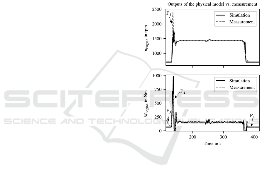
minal tractor. To gain an understanding of the causes
of the errors, an analysis of the simulation results was
carried out. Two significant causes of failure were
detected. Figure 8 presents a first excerpt of the mea-
sured test drives of the LNG-powered terminal tractor
and demonstrates both types of failure. As the po-
sitions P
1
in figure 8 show, one cause of failure can
be vehicle standstill, where the engine load is inde-
pendent of the input data and deviates from the usual
loads. In addition, errors may occur if the estimated
gear differs from the measured gear (see P
2
), resulting
in a different gear ratio.
Figure 8: Measured and simulated n
Engine
and M
Engine
dur-
ing a test drive of the LNG-powered terminal tractor.
The next step is to identify the unknown rolling
resistance coefficient f
R,Trailer
of the trailer model. To
do this, both, the measured data and the informa-
tion from the terminal operating system are linked
together. Then the internal structure of the ANNs
in the black box model of the combustion engine in
each powertrain has to be determined and data sets
for training, testing and validation have to be created.
Next, suitable hyperparameters of the ANNs must be
found by hyperparameter optimization. Afterwards
the accuracy of each ANN must be verified. Finally,
the physical model and the black box model for each
powertrain must be linked together and the accuracy
of each complete model must be examined. The com-
plete models can then be used to predict and discuss
the fuel consumption and exhaust emissions of the
fleet of terminal tractors at duisport for the diesel- and
LNG-powered powertrain.
Evaluation of Alternative Propulsion Concepts for Mobile Machinery: A Modelling Approach using the Example on LNG-powered Port
Handling Equipment
231

ACKNOWLEDGEMENTS
The work presented here was carried out within the
framework of the research project LeanDeR. This
project was funded by the European Regional De-
velopment Fund (ERDF) and the state government of
North Rhine-Westphalia, Germany.
REFERENCES
Abdelghaffar, W., Osman, M., Saeed, M., and Abdelfatteh,
A. (2002). Effects of Coolant Temperature on the Per-
formance and Emissions of a Diesel Engine. Ameri-
can Society of Mechanical Engineers, Internal Com-
bustion Engine Division (Publication) ICE, 38.
Abdullah, N., Ismail, H., Michael, Z., Abdullah, A. R., and
Sharudin, H. (2015). Effects of air intake tempera-
ture on the fuel consumption and exhaust emissions
of natural aspirated gasoline engine. Jurnal Teknologi,
76:25–29.
Dubois, G. (2018). Modeling and Simulation: Challenges
and Best Practices for Industry. CRC Press.
Duisburger Hafen AG (2019).
European Commission (2018). A Clean Planet for all. A
European strategic long-term vision for a prosperous,
modern, competitive and climate neutral economy.
European Parliament and the Council (2017). Commission
Delegated Regulation (EU) 2017/654 of 19 Decem-
ber 2016. Official Journal of the European Union, L
102:1–333.
Federal Ministry for the Environment, Nature Conservation
and Nuclear Safety (2019). Climate Action in Figures.
Facts, Trends and Incentives for German Climate Pol-
icy.
Geimer, M. and Pohlandt, C. (2014). Grundlagen mo-
biler Arbeitsmaschinen, volume 22 of Karlsruher
Schriftenreihe Fahrzeugsystemtechnik / Institut für
Fahrzeugsystemtechnik. KIT Scientific Publishing,
Karlsruhe.
Guzzella, L. and Onder, C. (2010). Introduction to Model-
ing and Control of Internal Combustion Engine Sys-
tems. Springer-Verlag Berlin Heidelberg.
Haken, K.-L. (2015). Grundlagen der Kraftfahrzeugtech-
nik. Carl Hanser Verlag.
Helms, H., Jamet, M., and Heidth, C. (2017). Renewable
fuel alternatives for mobile machinery. Technical re-
port, Institut für Energie- und Umweltforschung Hei-
delberg.
Hussain, J., Palaniradja, K., Natarajan, A., and Manimaran,
R. (2012). Effect of exhaust gas recirculation (EGR)
on performance and emission characteristics of a three
cylinder direct injection compression ignition engine.
Alexandria Engineering Journal, 51:241–247.
International Energy Agency (2019). CO2 Emissions From
Fuel Combustion 2019.
Jeoung, D., Min, K., and Sunwoo, M. (2020). Automatic
Transmission Shift Strategy Based on Greedy Algo-
rithm Using Predicted Velocity. International Journal
of Automotive Technology, 21(1):159–168.
Lajunen, A., Sainio, P., Laurila, L., Pippuri-Mäkeläinen, J.,
and Tammi, K. (2018). Overview of Powertrain Elec-
trification and Future Scenarios for Non-Road Mobile
Machinery. Energies, 11:1184.
Luz, R. (2015). Simulationsbasierte Methode zur Zerti-
fizierung der CO
2
Emissionen von schweren Nutz-
fahrzeugen. PhD thesis, TU Graz.
Milojevi
´
c, S., Skrucany, T., Milosevic, H., Stanojevic, D.,
Panti
´
c, M., and Stojanovic, B. (2018). Alternative
Drive Systems and Environmentaly Friendly Public
Passengers Transport. 3:105–113.
Mitschke, M. and Wallentowitz, H. (2014). Dynamik der
Kraftfahrzeuge. Springer Fachmedien Wiesbaden.
Mohan, G., Assadian, F., and Longo, S. (2013). Compar-
ative analysis of forward-facing models vs backward-
facing models in powertrain component sizing.
Schramm, D., Hesse, B., Maas, N., and Unterreiner, M.
(2020). Vehicle Technology - Technical Foundations
of Current and Future Motor Vehicles. De Gruyter
Oldenbourg, Berlin / Boston.
Schramm, D., Hiller, M., and Bardini, R. (2018). Vehicle
Dynamics. Springer, Berlin / Heidelberg, 2 edition.
Serikov, S. (2010). Neural network model of internal com-
bustion engine. Cybernetics and Systems Analysis,
46:998–1007.
Terberg Benschop (2015). YT222 LNG, 4x2. Technical
Specification.
Verein Deutscher Ingenieure e.V. (2016). VDI 4465
Blatt 1: Modellierung und Simulation - Modellbil-
dungsprozess.
Wipke, K., Cuddy, M., and Burch, S. (1999). Advisor 2.1:
A user-friendly advanced powertrain simulation using
a combined backward/forward approach. Vehicular
Technology, IEEE Transactions on, 48:1751 – 1761.
Xu, X. P. (1997). Experimental Modeling of A Hydraulic
Load Sensing Pump using Neural Networks. PhD the-
sis, University of Saskatchewan.
Zhao, N., Liu, Y., Mi, W., Shen, Y., and Xia, M. (2020).
Digital Management of Container Terminal Opera-
tions. Springer Singapore.
SIMULTECH 2020 - 10th International Conference on Simulation and Modeling Methodologies, Technologies and Applications
232
