Control of Sewer Flow using a Buffer Tank
K. M. Nielsen
1
, T. S. Pedersen
1
, C. Kallesøe
1
, P. Andersen
2
, L. S. Mestre
2
and P. K. Murigesan
2
1
Automation & Control, Department of Electronic Systems, Aalborg University, Aalborg, Denmark
2
Control & Automation, Aalborg University, Denmark
Keywords:
Sewer Flow Modelling, Model Predictive Control.
Abstract:
Flow variations of the inlet to a wastewater treatment plant (WWTP) are problematic due to the biological
purification process. A way to reduce variations from industrial areas is to insert a buffer tank. Traditionally
the only on-line measurement is the inlet flow to the wastewater treatment plant and reliable measurements in
the system are difficult to establish. A control scheme using only one on-line measured variable is shown to
be able to give considerable reduction in the flow variations. To implement the control scheme two models
are introduced. A linear model (delay model) from the buffer tank to the wastewater treatment plant and an
autonomous model describing the daily variations in the household sewer flow. A Model Predictive Controller
has been designed and tested in a laboratory set-up with good results.
1 INTRODUCTION
The topic within this paper is flow control for opti-
mization of wastewater treatment systems. The sewer
system drains wastewater from industries and pri-
vate households. A sewer system network consists
of gravity pipes, pressurized pipes, pumps, manholes,
weirs etc. making up a complex system. In this work,
the sewer network in the Danish city Fredericia with
approximately 50000 inhabitants is in focus.
The wastewater is comprised of different pollu-
tants like phosphor, nitrogen and biologically degrad-
able components characterized by Chemical Oxygen
Demand (COD). The inlet to the WWTP is varying
due to daily variations in household wastewater, vary-
ing industrial outlets and different time delays from
these sources to the WWTP inlet. In addition, precip-
itation causes irregular variations. In Fredericia in dry
periods 60 % to 70 % of the wastewater comes from
industries. The sewer system as well as the biologi-
cal processes are complex and further it is difficult to
make on-line measurements of the pollutants. A de-
tailed description of all phenomena is extremely com-
prehensive as seen in e.g. the simulation tool WATS
(T. Hvitved-Jacobsen et al., 2013),(DHI, 2017) and is
not well suited for controller design. In this work,
only COD is taken into account and furthermore it
is assumed that no biological processes takes place
in the sewer network. Therefore, a simple model de-
scribing the main dynamics is formulated.
In Fredericia the only available real time on-line
measurement is the inlet flow to the WWTP. Off-
line measurements of COD, nitrate and phosphor are
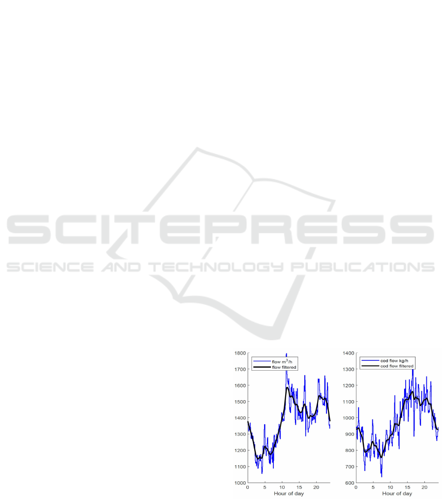
available from October 2017. The average and fil-
tered average of the total flow as well as the COD
flow in October 2017 are shown in Fig.1. Flow and
COD measurements are sampled from the inlet to the
WWTP. As seen in Fig.1 the shape of the COD and
flow inlet are similar, therefore only control of the
flow to WWTP is investigated in this work. Varia-
tion in the COD-flow can be considered in a similar
way and will be considered in a continuation of the
work.
Figure 1: 24 hours average flow and COD based on mea-
surements from 30 days at the inlet to Fredericia WWTP.
(Schlutter, 1999). Here, it is assumed there is no infiltration
by the groundwater into the sewer system.
Nielsen, K., Pedersen, T., Kallesøe, C., Andersen, P., Mestre, L. and Murigesan, P.
Control of Sewer Flow using a Buffer Tank.
DOI: 10.5220/0009871300630070
In Proceedings of the 17th International Conference on Informatics in Control, Automation and Robotics (ICINCO 2020), pages 63-70
ISBN: 978-989-758-442-8
Copyright
c
 2020 by SCITEPRESS – Science and Technology Publications, Lda. All rights reserved
63

A way to minimize the flow variations is to insert
buffer tanks in the sewer network and control the out-
puts from these. At the moment no buffer tanks are
available in the sewer system in Fredericia but are to
be planned. A logical place for a buffer tank is close
to the industrial outlets. An algorithm to control the
outflow from the buffer tank in order to minimize flow
variations at the inlet to WWTP is developed. Control
of sewer systems are described in (Ocampo-Martinez,
2005), (Marinaki and Papageorgiou, 2005), (Over-
loop, 2006), (Pilgaard and Pedersen, 2018), (Mestre
and Murugesan, 2019).
To design a controller, models of the buffer tank,
the sewer network, the household flows and industrial
flows are necessary.
A simple tank model based on a mass balance is
used. A dynamic model describing main character-
istics of the sewer network is formulated; here it is
shown that the Saint-Venant equations under certain
assumptions can lead to a delay model. The model
describing the flows from households to the WWTP
is an autonomous state space model where the coef-
ficients are based on the Fourier transform of mea-
surements from one month Fig. 1. The outflow from
industry is estimated from 24 hours measured time se-
ries.
A Model Predictive Controller (MPC) with a per-
formance function aiming to minimize the variance
of inlet flow to the WWTP has been formulated given
buffer tank volume constraints.
To test the benefit of a buffer tank inserted in the
sewer system a laboratory setup (Smart Water Lab) is
used.
In section 2 the Fredericia sewer system is de-
scribed. Section 3 considers the control concept. The
sewer system modelling is described in section 4.
Section 5 is a description of the actual control of the
buffer tank output. The control concept is tested in the
laboratory which is described in section 6 and finally
the conclusion is in section 7.
2 FREDERICIA SEWER SYSTEM
Fredericia wastewater treatment plant covers the town
of Fredericia, nearby villages and industrial areas
north and west of the town. The total sewer net is
among the largest in Denmark. Households and in-
dustrial areas north and west of the town dominate the
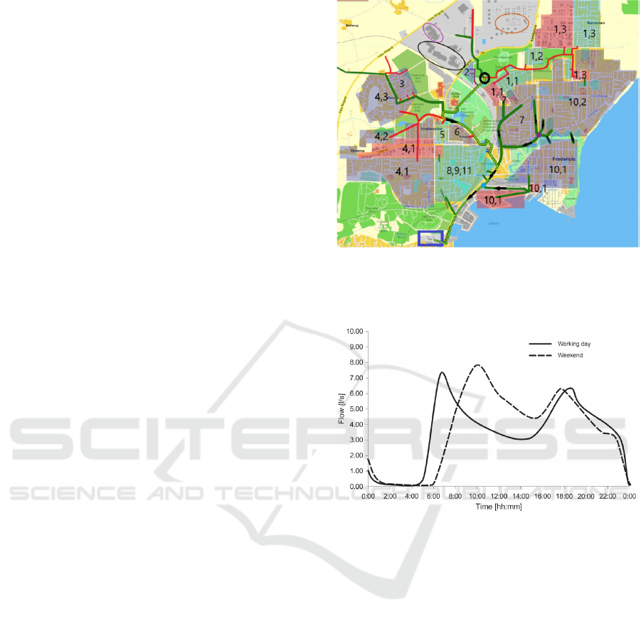
wastewater in Fredericia. The map shows the north-
ern part of Fredericia divided in subareas. A large
number of pipes leads to the WWTP. In this work, the
pipes from the industrial areas to the WWTP are con-
sidered. These are indicated in the map Fig. 2.
Figure 2: Main sewer system in Fredericia, (Pilgaard and
Pedersen, 2018). The blue square is the WWTP, oval shapes
are industrial areas, black circle is inlet from industry to the
main pipe.
Figure 3: 24 hours average household flow from 2000 in-
habitants Wastewater production from a small village Fre-
jlev, Denmark, Here, it is assumed there is no infiltration by
the groundwater into the sewer system (Schlutter, 1999).
Household wastewater is predictable with regard
to flow. Fig. 3 shows typical average emission from
2000 inhabitants in an area without industries. As
seen in Fig. 2, the area covered by the wastewater
plant is large and the sewer network is split into nu-
merous branches implying that the shape of the inflow
from the households to the wastewater treatment plant
is influenced by varying delays in flow.
In the WWPT, the quality of the wastewater treat-
ment and biogas production are dependent on the in-
flow, as the biological processes need time for scal-
ing. Control of the inlet flow will potentially improve
the quality of the WWTP processes. A case study
with one industrial plant is investigated; it comprises
one buffer tank placed close to the industrial plant,
the sewer network from the buffer-tank to the WWTP
and one model for the entire household flow to the
WWTP.
ICINCO 2020 - 17th International Conference on Informatics in Control, Automation and Robotics
64

3 CONTROL CONCEPT
The main goal for the control system is to reduce the
fluctuations in the inlet flow, Y , to the WWTP. The as-
sumptions are that the only measurement is Y and the
only controllable variable is the outlet flow U from
the buffer tank. The inlet flow from industries to the
buffer tank is Q
i
. Y
re f
is the WWTP inlet flow refer-
ence. In this work, we look at one buffer tank. The
concept for controlling this may easily be extended to
more detention tanks. In Fig. 4 shows a sketch of the
simplified system.
Figure 4: Simplified sewer system with the main compo-
nents buffer tank, households, sewer pipe and WWTP.
A classical control concept is illustrated in Fig.
5. Q
h
is the total household flow disturbance and is
seen as a flow directly to the WWTP. The model of
the main pipe may include a transport delay; there-
fore, a classic controller will result in a low bandwidth
and poor disturbance rejection (Aastrom and Haeg-
glund, 2006), (Postlethwaite and Skogestad, 2005).
The disturbance is periodic, see Fig.3, this periodic-
ity is difficult to include in a classic control concept.
It is well known from the classical control theory that
cascading can improve the performance. More flow
measurements in the main pipe will make this pos-
sible and up-stream measurements of the household
flow could be used as feed forwards. Iterative learn-
ing control could be another way to improve a clas-
sic controller and a third concept is to use a neural
network. Model Predictive Control (MPC) relies on
predictions of future system behavior. In this case
household wastewater flow shows periodicity and the
delay times in the sewer net can be found, therefore
the MPC method is chosen.
+
ref
Q
h
U Y
Controller Main pipe
+
−
+
Y
Figure 5: Classical control concept for the problem showing
inputs, outputs and disturbances.
4 MODELLING THE SEWER
SYSTEM
The model for the MPC consists of a tank model, a
model of the sewer network, a household disturbance
model and a description of the industrial wastewater
flow.
The Tank Model
The tank is modelled as an integrating system
ρdV (t)
dt
= ρQ
i
(t) − ρU(t) (1)
Where V is the volume of wastewater in the tank
and ρ is the density. It is assumed that ρ is a constant.
The discrete version is:
V (k + 1) = V (k) + T
s
(Q
i
(k) −U (k)) (2)
Where T
s
is the sample time.
The Sewer Network Model
The pipes are generally not filled and considered as
open channels. The flow and the level in sewer net-
works are usually modelled by the Saint-Venant equa-
tions (Crossley, 1999), (frese.dk, 2018), (Andersen,
1977), (Michelsen, 1976). The general form of the
Saint-Venant equations are
∂A
∂t
+
∂Q
∂x
= 0 (3)
1
gA
∂Q
∂t
+
1
gA
∂
∂x
(
Q
2
A
) +
∂h
∂x
+ S
f
− S
b
= 0 (4)
where Q is the sewage flow [m
3
/s], A is the cross-
sectional area of the sewage flow [m
2
], h is the level
in the pipes [m], S
b
is the slope and S
f
is the fric-
tion. x is a spatial variable measured in the direction
of the flow [m], t is time [s] and g is gravitational ac-
celeration [m/s
2
]. If COD is included in the control a
supplementary equation is used to describe this.
These equations are not linear and thereby not
well suited for MPC. A simplified linear model is de-
rived.
The transport of fluids could also be seen as a
wave propagation. Since there is a net mass transfer
involved, the waves are translational. To understand
the wave phenomena in gravity and pressure driven
fluid mass flows, kinematic wave or dynamic wave
analysis is important. When the inertial and pressure
forces are minor in the momentum equation (4), kine-
matic waves govern the flow. Dynamic waves govern
Control of Sewer Flow using a Buffer Tank
65

flow when these forces are dominating. In a kine-
matic wave, the flow does not accelerate considerably
as the gravity and friction forces neutralize each other.
Disregarding the first three terms in equation (4),
the remaining two terms can be replaced by a flow
expression for a fully filled pipe; Mannings equation,
(R. Manning and Leveson, 1890) gives a relation be-
tween A, h and Q. Since cross sectional area is related
to water depth A = A(h) the following relation can be
given Q = Q(h) .
Using the chain-rule for the continuity equation
(3):
∂A
∂h
∂h
∂t
+
∂Q
∂h
∂h
∂x
= 0 (5)
The two terms
∂Q
∂h
and
∂A
∂h
can be expressed using
the Manning equation. These terms are non-linear.
Here we use a linearized version of this equation and
apply small fluctuations to the flow Q and thereby to
the water level h. This leads to the relation
c =
∂Q
∂A
=
∂Q
∂h
∂A
∂h
(6)
and the equation
∂h
∂t
+ c
∂h
∂x
= 0 (7)
close to the operating point
∂Q
∂h
is constant giving:
∂Q
∂t
+ c
∂Q
∂x
= 0 (8)
This equation describes waves propagating with
unchanged shape and speed c. Changes of flow at the
inlet of a pipe will appear at the outlet after a time
delay T
d
corresponding to the pipe length and propa-
gation speed c. This can be verified by assuming that
the flow in position x = 0 is Q(0,t) and is known as a
function of time t. The flow in an arbitrary position x
at time t −
x
c
is assumed to be
Q(x,t) = Q(0,t −
x
c
) (9)
To show that this is a solution to equation 8, the
partial derivatives with respect to t and x is
∂Q
∂t
=
∂Q(0,t −
x
c
)
∂(t −
x
c
)
∂(t −
x
c
)
∂t
=
∂Q(0,t −
x
c
)
∂(t −
x
c
)
(10)
∂Q
∂x
=
∂Q(0,t −
x
c
)
∂(t −
x
c
)
∂(t −
x
c
)
∂x
=
∂Q(0,t −
x
c
)
∂(t −
x
c
)

−1
c

(11)
inserting these two expressions into equation (8)
results in
∂Q(0,t −
x
c
)
∂(t −
x
c
)
+ c
∂Q(0,t −
x
c
)
∂(t −
x
c
)

−
1
c

= 0 (12)
which satisfies the equation.
These calculations show that the flows in the
sewer network can be modelled as delays under the
given assumptions.
The output flow from the buffer tank U is de-
layed by
L
c
where L is the length of the pipe from the
buffer tank to the WWTP. For control purposes the
discretized U can be expressed as U(k − τ) where τ is
the transport delay
The total flow to the WWTP Y is the household
flow and the delayed flow from the buffer tank, Y can
be described as:
Y (k) = Q
h
(k) +U (k − τ) (13)
where Q
h
(k) is the household flow at time k.
The Household Disturbance Model
The purpose of the model is to estimate the future
household flow. Investigations have shown a 24 hours
pattern where the flow is low during the night, Fig. 3.
A way to find the model of the flow is to use a large
number of measurements to find the frequency spec-
trum. Here the spectrum is found using a DFT and the
complex coefficients are used in an autonomous state
space model which describes average daily household
flow. This model supplemented with a stochastic in-
put will be used in a Kalman observer.
A continuous time sinusoidal in amplitude phase
form is described by (Kuo, 1966)
y(t) = a
0
+ a · cos(ωt + φ) (14)
where a
0
is the mean or zero frequency term, a is
the amplitude, ω is the frequency and φ is the phase
difference.
An autonomous state space model (SSM) can be de-
fined
˙x = Ax (15)
y = Cx (16)
whose state vector, system matrix, input and out-
put matrix are
x(t) =


a
0
a · cos(ωt + φ)
a · sin(ωt + φ)


(17)
and
ICINCO 2020 - 17th International Conference on Informatics in Control, Automation and Robotics
66

A =


0 0 0
0 0 −ω
0 ω 0


, C =

1 1 0

(18)
y(ω) is the Fourier transform of y(t). The real part
and the imaginary part of the Fourier transform coef-
ficients are used in C. The above SSM contains just
a single frequency. When there are multiple frequen-
cies, the sinusoidal signal and SSM is:
y(t) = a
0
+
N
∑
n=1
a
n
· cos(nωt + φ
n
) (19)
x(t) =



















a
0
a
1
· cos(ω
1
t + φ
1
)
a
1
· sin(ω
1
t + φ
1
)
a
2
· cos(ω
2
t + φ
2
)
a
2
· sin(ω
2
t + φ
2
)
.
.
.
.
.
a
k
· cos(ω
k
t + φ
k
)
a
k
· sin(ω
k
t + φ
k
)



















A =



0 0 0 0
0 A
1
0 ...
0 0 A
2
...
. . . A
k



where
A
i
=

0 −ω
i
ω
i
0

i = 1,2 ... k
C =

1 1 0 1 0 ... 1 0

The discrete-time equivalent of A in (18), with
sampling time T
s
is
Φ(T
s
) = e
AT
s
(20)
This matrix has block diagram structure,
Φ(T
s
) = diag(Φ
0
(T
s
),Φ
1
(T
s
),·· · ,Φ
k
(T
s
)) (21)
and can be split into
Φ
0
(T
s
) = 1 (22)
Φ
i
(T
s
) =

cos(ω
i
T
s
) −sin(ω
i
T
s
)
sin(ω
i
T
s
) cos(ω
i
T
s
))

(23)
Model for Industrial Waste Water
The industrial wastewater flow Q
i
is a significant part
of the total inlet to the WWTP. The flow is varying
and large COD pulses occur. Q
i
is measured several
times off-line one day per month.
Information on the industrial wastewater flow is
relevant for control purposes. The best-case scenario
is exact knowledge of flow and COD from the indus-
trial companies, alternatively a model for typical Q
i
variations can be of use. A third method is on-line
measurement of the COD and level in the buffer tank
inserted close to industry. To prove the concept Q
i
is
modelled as a constant flow combined with different
flow variations.
Model Parameters for Fredericia Sewer
System
The sewer network model from the buffer tank to the
WWTP is simplified to a time delay. This delay is
found using cross correlation of data from one day
from the heavy industry and data from the inflow to
the WWTP. It turns out that the strongest correlation
is at approximately 100 minutes. To find the param-
eters in the household disturbance model, measure-
ments of 30 days inflow to the WWTP are used. The
30 days measurement has been digital Fourier trans-
formed and the power spectrum is shown in Fig. 6.
Power Spectrum of Y(t)
0 0.005 0.01 0.015 0.02 0.025 0.03 0.035 0.04 0.045
Frequency (Hz)
0
1
2
3
4
5
6
7
8
9
10
|P(f)|
10
4
Figure 6: Bar plot of power spectrum which is the square of
DFT’s magnitude. At low frequencies, the magnitudes are
large.
The dominating frequencies are found by using a
threshold in the power spectrum. In Fig. 7 frequen-
cies from three different thresholds are simulated.
5 CONTROL OF THE BUFFER
TANK OUTPUT
The MPC (Maciejowski, 2002) aims to minimize the
variance of the input flow to WWTP. The following
performance function is used:
J =
H
p
∑
k=1

ˆ
Q
h
(k + τ) +U(k) − µ

2
R
+
H
p
∑
k=1

µ

S
(24)
Control of Sewer Flow using a Buffer Tank
67

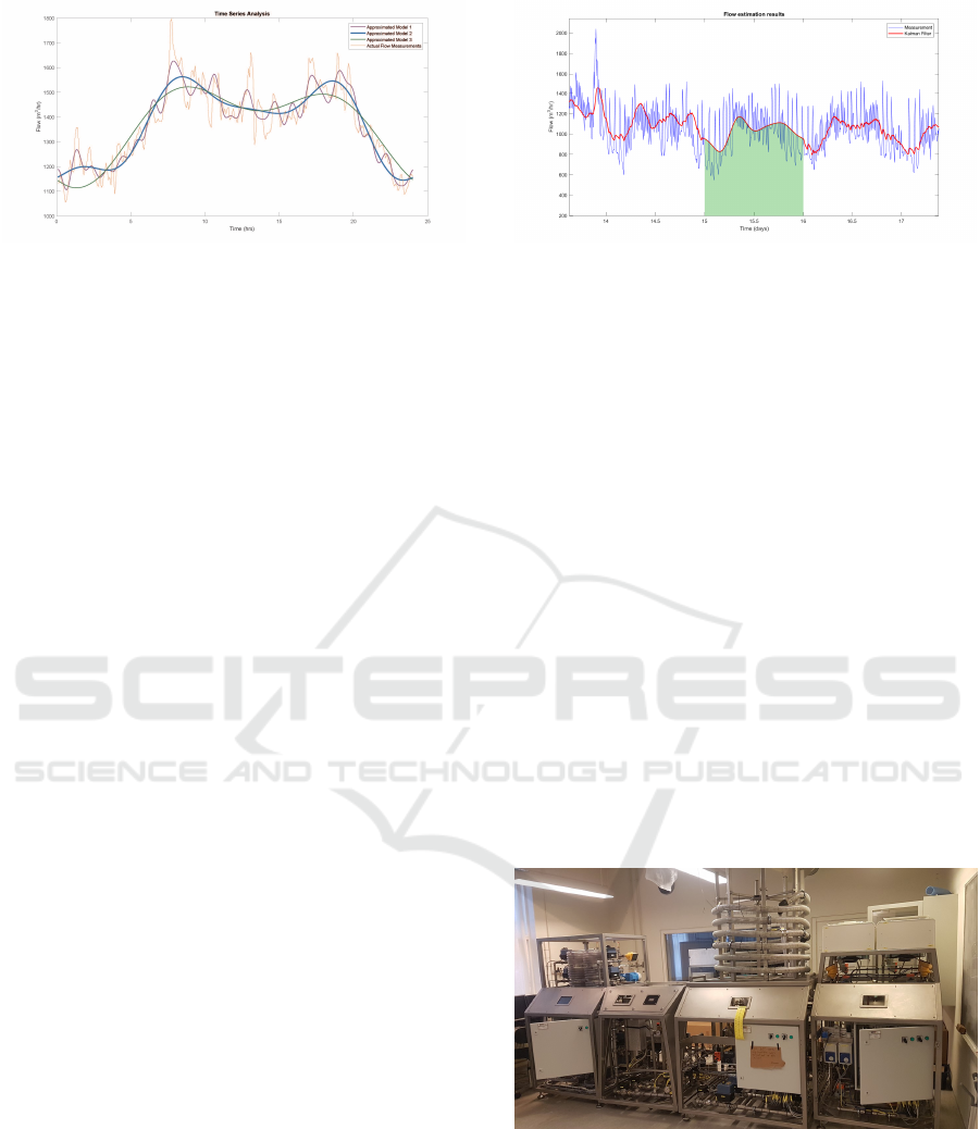
Figure 7: Different model approximations of the original
flow data. The thresholds set for the model 1, 2 and 3 are
respectively 2500, 900 and 400. The purple curve consid-
ered 10 frequencies in the model. The blue curve considered
only 5 frequencies in the model. The latter model is used in
the subsequent section.
subject to system dynamics and constraints
V (k + i + 1) = V (k + i) + T
s
(
ˆ
Q
i
(k + i) −U(k + i))
Y (k + i + τ) =
ˆ
Q
h
(k + i + τ) +U(k + i)
V
min
≤ V ≤ V
max
U
min
≤ U ≤ U
max
(25)
The first equation is the model of the buffer tank,
where
ˆ
Q
i
is a prediction of the industrial outlet. In the
performance function the first term is the variance of
the total input to the WWTP, Y . µ is the mean value,
H
p
is the prediction horizon.
ˆ
Q
h
is the estimated out-
put of the household flow.
Estimation of
ˆ
Q
h
is based on a Kalman filter
(Kalman, 1960) assuming noise added to the au-
tonomous household flow model.
X(k + 1) = ΦX(k) + K(Q
h
(k) −CX(k)) (26)
where K is the Kalman-gain. The household flow
is predicted by
X(i + 1) = ΦX(i)
ˆ
Q
h
(i) = CX(i)
(27)
for
i = k..(k + H
p
+ τ) (28)
The Kalman filter approach is tested using mea-
sured data from Fredericia. In Fig. 8 the blue curve
represents measured data, the red curve is the Kalman
estimate. The Kalman filter is updated with measure-
ments at each sample except in the green region. In
the green section the Kalman filter estimates without
measurements. The results are good within the 24
hours estimate without measurements. The data rep-
resents a day without precipitation and the estimate
will be uncertain in rainy periods.
Figure 8: The Kalman filter estimation of
ˆ
Q
h
for day 15.
The process noise and measurement noise in the Kalman
filter had a variance of 0.01 and 25 respectively.
6 LABORATORY TEST OF THE
CONTROL CONCEPT
A buffer tank and on-line measurements are to be im-
plemented in Fredericia. To prove the concept the
control system is tested in Smart Water Lab at Aal-
borg University seen in Fig.9. Smart Water Lab has
components as tanks, pumps, valves, gravity pipes,
pressurized pipes etc. The modules of the Smart Wa-
ter Lab are configured to emulate the simplified sys-
tem as in Fig. 10. The consumer station is a buffer
tank from which appropriate household flow is emu-
lated. The blue arrows are pipes in the sewer system
and the sewer station is the WWTP. The purpose of
the pumping station is twofold, firstly it generates a
disturbance flow to the inlet of the Sewer Station emu-
lating the household flow and secondly it re-circulates
water to the consumer tank (yellow arrow).
Figure 9: Smart Water Lab at Aalborg University.
Deterministic (white-box) models are developed
to describe the dynamics of some key components of
the sewer network.
The laboratory set-up simulates the delay in the
gravity pipe and it is possible to introduce a distur-
bances illustrating the periodic household flow. The
disturbance can be seen as the yellow curve in Fig.
11. The flow from industry is implemented as a con-
ICINCO 2020 - 17th International Conference on Informatics in Control, Automation and Robotics
68

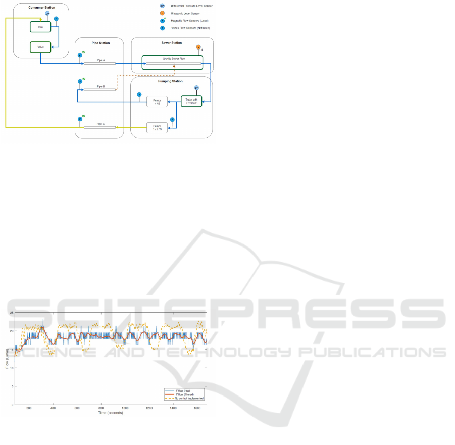
Figure 10: Circuit for the test set-up in Smart Water Lab
containing a consumer station, a pipe station, a sewer station
and a pumping station.
stant flow to the buffer tank. An MPC minimizing the
performance function equation 24 is implemented in
the laboratory by use of YALMIP (M.C. Grant and
Stephen, 2014), (Lofberg, 2014). It aims to minimize
the variations of the inlet flow to the sewer station.
The result can be seen in Fig. 11. The measurement
of the controlled flow (blue) has poor resolution, a fil-
tered version is the red curve. It is seen that the con-
trolled inlet flow has a lower variance than the original
uncontrolled flow (yellow).
Figure 11: Comparison of uncontrolled (yellow) and con-
trolled (blue and red) inlet to the sewer station.
The laboratory test shows that a buffer tank in
combination with an MPC algorithm can reduce the
variations in the inlet flow to the WWTP.
7 CONCLUSION
Typical inlet to a WWTP consists of periodic house-
hold flow and industrial flow. A control system for
minimization of flow variations to a WWTP using
a buffer tank for the industrial flow has been con-
structed. The controller is based on two models, one
model describing the flow variations from the buffer
tank to the WWTP and one describing the household
flow. The flow from the buffer tank to the WWTP is
described by the Saint-Venant equations. Under linear
assumptions it is shown that the flow model results in
a time delay. The model for the household flow uses
an autonomous description. The two models are in-
serted in a MPC with a performance that minimize
the flow variations. A lab set-up shows that the con-
trol concept is able to minimize the variance of the
mentioned flow.
REFERENCES
Aastrom, K. J. and Haegglund, T. (2006). Avanced PID
contro l. ISA.
Andersen, P. (1977). Optimering af driftsbetingelser for
spildevandsanlæg gennem automatisering. Aalborg
University, Denamrk.
Crossley, A. J. (1999). C, Accurate and efficient numeri-
cal solutions for the Saint Venant equations of open
channel flow. University of Nothingham.
DHI (2017). Wats-wastewater aeronoc/anaerobic transfor-
mation in sewers, mike eco lab template. In Scientific
Description. MIKE.
frese.dk (2018). https://www.frse.dk/Fredericia-
spildevand.aspx. urldate: 2018-10-03.
Kalman, R. E. (1960). A new approach to linear filtering
and prediction problems,Journal of basic Engineering
vol2, nr1, p 35-45. American Society of Mechanical
Engineers.
Kuo, F. F. (1966). Network analysis and synthesis. John
Wiley and Sons.
Lofberg, J. (2014). A toolbox for modeling and optimiza-
tion in MATLAB. CACSD Conference, vol.3, Taipei,
Taiwan.
Maciejowski, J. M. (2002). Predictive control: with con-
straints. Pearson education.
Marinaki, M. and Papageorgiou, M. (2005). Optimal real-
time control of sewer networks. Springer Science &
Business Media.
M.C. Grant, S. B. and Stephen, P. (2014). The
CVX Users Guide, Release 2.1. URL http://cvxr.
com/cvx/doc/CVX.
Mestre, L. S. and Murugesan, P. K. (2019). Laboratory Em-
ulation and Control of a Sewer System with Storage,
Master Thesis, Control and Automation, Aalborg Uni-
versity. Aalborg University, Denmark.
Michelsen, H. (1976). Ikke-stationær strømning i
delvis fyldte kloakledninger: en dimensioneringsme-
tode og en analysemetode. Afdelingen for Jord-
og Vandbygning, Den kgl. Veterinaer-og Landboho-
jskole,Denmark.
Ocampo-Martinez, C. (2005). Model predictive control of
wastewater systems. Springer Science & Business
Media, 2.
Overloop, P. J. V. (2006). Model predictive control on open
water systems. IOS Press.
Pilgaard, T. H. and Pedersen, J. N. (2018). Model Predictive
Control of a Sewer System, Master Thesis, Control
Control of Sewer Flow using a Buffer Tank
69

and Automation, Aalborg University. Aalborg Uni-
versity, Denmark.
Postlethwaite, I. and Skogestad, S. (2005). Multivariable
Feedback Control- Analysis and Design. Wiley and
Sons Ltd.
R. Manning, J. P. Griffith, T. P. V.-H. and Leveson, F.
(1890). On the flow of water in open channels and
pipes.
Schlutter, F. (1999). Numerical modelling of sediment
transport in combined sewer systems, The Hydraulics
and Coastal Engineering Group, Dept. of Civil Engi-
neering. Aalborg University.
T. Hvitved-Jacobsen, J. Vollertsen, and A. H. Nielsen
(2013). Sewer processes: microbial and chemical pro-
cess engineering of sewer networks. TCRC press.
ICINCO 2020 - 17th International Conference on Informatics in Control, Automation and Robotics
70