Performance Analysis of the Force Control for an Electromechanical
Feed Axis with Industrial Motion Control
Andre Sewohl
1
, Manuel Norberger
1
, Chris Schöberlein
1
, Holger Schlegel
1
and Matthias Putz
1,2
1
Institute of Machine Tools and Production Processes, Chemnitz University of Technology, Reichenhainer Straße 70,
09126 Chemnitz, Germany
2
Fraunhofer-Institut for Machine Tools and Forming Technologies, Reichenhainer Straße 70, 09126 Chemnitz, Germany
Keywords: Electromechanical Feed Axis, Motion Control, Force Control, Controller Design, Controller Performance.
Abstract: Control of process forces provides significant economic benefits for many use cases. The force is often the
limiting factor for the design of the processes and the choice of parameters. As a controlled variable, it is
predestined to ensure stability and safety of many processes. Direct influence also enables increasing
productivity and improving part quality. However, force control has not yet become established for
manufacturing processes in machine tools with electromechanical axes and industrial control. A major
problem area is the lack of real-time capability. Due to the delay times in signal processing, real-time
capability is not guaranteed for dynamic movements of feed axes. High-resolution and fast measurement
inputs are particularly relevant here. Industrial control manufacturers have made significant progress in this
area. In this publication, the experimental setup of an electromechanical feed axis is presented, which is
equipped with new industrial control components. The implementation of the force control is also described.
Focus is on the investigations regarding the controller performance. The set point and disturbance behaviour
as well as the reaction to the process start are considered.
1 INTRODUCTION
In modern production systems, there is a trend to
replace mechanical motion solutions with electrical
ones. There are many strategies for controlling
machine-specific quantities, such as the position or
speed of electromechanical axes. The concept of
cascade structure, also called servo control, has
become established in this field (Schröder, 2001).
The use of controlled electromechanical drive
systems can meet the increasing demands on the
machines in terms of dynamic behavior, as well as
higher productivity and accuracy.
Nevertheless, in the area of production
engineering, there are ongoing efforts to improve
manufacturing strategies and processes in terms of
stability, quality and efficiency. One possibility for
ensuring stable process conditions and reducing
rejected parts is closed loop control of quality
determining parameters (Allwood et al., 2016). The
development of suitable control concepts at the
process level, in which significant process variables
are taken into account as controlled values, offers
considerable scope for improvement at this point.
There are many process variables which have an
influence to the quality of a part. However, usually it
is very difficult to control these values. The
metrological acquisition of corresponding
parameters constitutes a further challenge.
The machining force is a suitable parameter that
can be detected well by measurement. It is of
particular relevance for the majority of processes in
the field of production technology. As a controlled
variable, it is predestined for ensuring process
stability and safety. Machining forces are often the
limiting factor for the design of the processes and
the choice of parameters. Excessive loads can cause
damage and defects to the workpiece, tool or
machine. In the worst case, they even lead to its
destruction. In addition, process forces provide
important information about the process state and
allow conclusions about deviations in the production
process, the machine, the tool, the workpiece or
material.
The next chapter provides an overview of the
state of the art in force control and research efforts.
Sewohl, A., Norberger, M., Schöberlein, C., Schlegel, H. and Putz, M.
Performance Analysis of the Force Control for an Electromechanical Feed Axis with Industrial Motion Control.
DOI: 10.5220/0009866806670674
In Proceedings of the 17th International Conference on Informatics in Control, Automation and Robotics (ICINCO 2020), pages 667-674
ISBN: 978-989-758-442-8
Copyright
c
 2020 by SCITEPRESS – Science and Technology Publications, Lda. All rights reserved
667

In addition, the existing challenges and the need for
action are shown. The selected test-setup is
presented in the third chapter. Subsequently,
performed experiments are explained and
consecutively evaluated. The last chapter completes
the publication with a summary and description of
the conclusions.
2 STATE OF THE ART
Control of process forces provides significant
economic benefits for many use cases by increasing
operation productivity and improving part quality.
Especially for processes in the field of machining
technology, targeted influencing of the process
forces is of outstanding importance (Ulsoy and
Koren, 1993). For this reason, a large number of
concepts and algorithms for control of process forces
have been investigated and developed both in
research and industry.
First significant ideas associated with process
control systems were introduced in the 1960’s
(Ulsoy and Koren, 1989). An early work
investigated a PID-structure with fixed gain
controller as approach. But it turned out that fixed-
gain controllers could not maintain system
performance and stability in machining force control
(Koren and Masory, 1981). That lead to an
increasing interest in the development of adaptive
machining force controllers. The majority of the
work in machining force control is devoted to the
subject of adaptive techniques. An overview to the
developments in adaptive control systems is given in
(Ulsoy et al., 1983). (Liu et al.; 2001) compares
different adaptive control techniques. However,
adaptive controllers can be difficult to develop,
analyze, implement, and maintain due to their
inherent complexity. Consequently, adaptive
machining force controllers have found little
application in industry (Landers et al., 2004).
In recent years, approaches with fuzzy logic
controllers have been increasingly investigated
(Zuperl et al., 2005), (Xu and Shin, 2008), (Kim and
Jeon, 2011). Artificial neural networks also came
into focus of considerations increasingly (Haber and
Alique, 2004), (Yao et al., 2013). Even a novel
approach using predictive algorithms was recently
presented in (Stemmmler et al., 2017). But these
concepts were also unable to establish themselves in
industry.
A key problem is that complex control structures
and algorithms are difficult to integrate in machine
tools with conventional industrial control.
Additional hardware usually has to be used. The
resulting communication times in turn reduce
performance and reaction speed is limited. Direct
access to the control level (e.g. the interpolation
cycle) is necessary to ensure real-time capability. In
this context, measuring the process forces with
additional sensors is also problematic. The cycle
time is increased even further through signal
processing and integration into the control system.
This becomes clear in (Posdzich et al., 2019) for
example. The system is superimposed to the control
and the entire measuring chain has a sampling time
of approximately 40 ms. The control can only react
to a limited extent to quickly acting disturbance
forces.
High-resolution measurement inputs are
particularly relevant for force control, besides real-
time capability. The configuration of the load cell
with strain gauges is based on maximum loads. As a
result, only a small part of the total area remains for
the force actually occurring in the process with
12-bit converters. Therefore higher resolutions
(16-24 bit) are necessary.
Industrial control manufacturers have made
significant progress in these areas. The control
components and assemblies from Beckhoff meet
these requirements and offer new opportunities. The
corresponding experimental test-setup for an
electromechanical axis is presented in the next
chapter. Here, the implementation options of direct
force control are considered and examined with
regard to their limits and performance.
With regard to the design of a force control on
electromechanical feed axes, no generally applicable
regulations are known yet. Accordingly, no auto-
tuning functionalities are available on the control
side. Since no automatism or reproducible procedure
can be applied, the usual practice of manual
parameterization is used first. In addition, various
setting rules are examined with regard to their
suitability.
3 TEST-SETUP
For the experiments, a test-setup of an
electromechanical feed axis was selected, which is
designed for loads up to 10 kN. The mechanical
construction and control engineering structure are
described below. The commissioning and
enhancement with a force control are elucidated, too.
ICINCO 2020 - 17th International Conference on Informatics in Control, Automation and Robotics
668

3.1 Structure of the Drive Train
The basic structure of the test-setup corresponds to a
portal construction. However, only one drive is used
to generate the movement. The selected standard
servomotor AM8031 is suitable for drive solutions
with highest demands on dynamics and
performance. The rotational movement of the motor
is transmitted to a gear via a drivebelt. Another belt-
gear connection is used to translate and split the
rotation between the two spindles, which are
integrated in the frame. The traverse is attached to
the two ball screws, which are arranged at the same
height. These are used to convert the rotation into a
translatory upward and downward movement.
Synchronism of the spindles and parallelism of the
traverse, which is used for load transfer, are
mechanically guaranteed with this construction. The
entire drive train with its single transmission
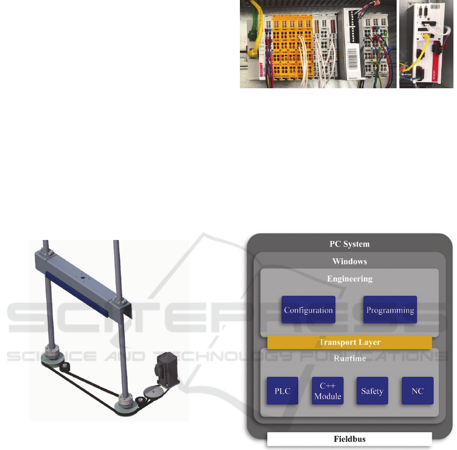
elements is illustrated as a CAD-model in Figure 1.
Figure 1: Drivetrain of the electromechanical axis.
3.2 Control Components
A digital compact servo controller of type AX5101
is used appropriate to the servo motor. The system is
also equipped with safety modules, analog and
digital I/O-modules, an ELM3502 terminal, a power
supply terminal and an EtherCAT bus coupler. All
components are connected via the backplane bus.
Communication with the servo controller and the
external PC takes place via the EtherCAT-
connection. This structure is illustrated in Figure 2.
The Software TwinCAT 3 (The Windows
Control and Automation Technology) automation
suite is available on the external PC. It is the core of
the control system and can be assigned to PC-based
Figure 2: Control engineering of the test-setup.
control technology. The TwinCAT software system
from Beckhoff converts almost any PC-based
system into a real-time control with several PLC,
NC, CNC or RC runtime systems. This software is
used, among other things, for programming,
configuration and control. The execution system and
the execution times can be freely defined and
program parts can be assigned to own tasks. The
basic architecture of TwinCAT is shown in Figure 3.
Figure 3: Twin-CAT architecture.
The recently developed ELM3502 terminal is of
particular importance in this assembly. It can be
used for the measurement bridge evaluation of full,
half or quarter bridges. An essential feature is the
high resolution of 24 bits with a very fast sampling
rate of 50 µs. This module is used to connect the
signals of the force sensor so that direct force control
can be implemented on the test-setup. A SSM-AJ-
10 kN force sensor from Interface, which is based on
strain gauge technology, is used for force
measurement.
Performance Analysis of the Force Control for an Electromechanical Feed Axis with Industrial Motion Control
669

3.3 Commissioning
During the commissioning of the test-setup, the
position control is first implemented to ensure basic
functionality. It is designed in a cascade structure.
The parameters are set from the inside out, starting
with the current control loop. This is based on the
performance data and electrical parameters of the
motor. The parameters of the current control loop
are already defined and set by the manufacturer.
Next, the velocity control loop is superimposed.
Autotuning algorithms for drive control are currently
still being developed at Beckhoff. Therefore, the
velocity controller is commissioned using the
Ziegler-Nichols method, which is frequently used in
practice. For this purpose, the gain factor of the
speed controller was increased up to the stability
limit. Then the gain to be set corresponds to 45 % of
the critical value. The reset time for the PI controller
corresponds to 85 % of the oscillation frequency.
The gain factor K
v
of the position controller is
calculated according to the specification of
(Zirn, 2008). This depends on the damping of the
system. With a damping value of 1, the system is not
vibratory. The following equation applies here:
K
v
= 1 / (4*T
e
q
,n
) (1
)
The equivalent time constant of the speed control
loop can be determined from the frequency response
using the following equation:
T
e
q
,n
= 1 / (2π*ω
b
) (2
)
The parameter ω
b
corresponds to the bandwidth
that is at the intersection of the amplitude response
with the -3dB line. The corresponding frequency
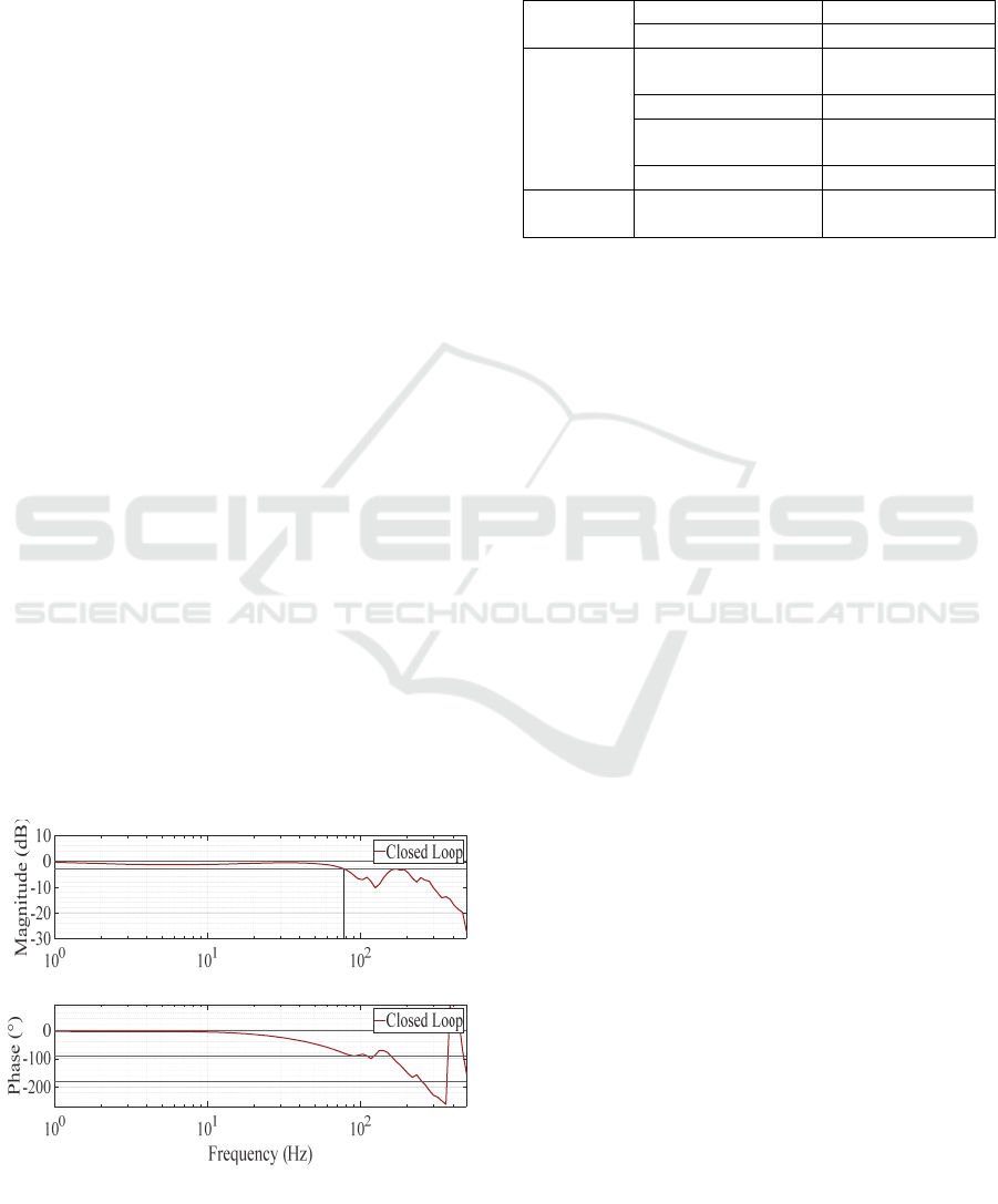
response is shown in Figure 4.
Figure 4: Frequency response of the velocity control loop.
The bandwidth is 78 Hz, which results in an
equivalent time constant of 2 ms. The gain factor K
v
is thus 125 s
-1
. The parameters of the cascade control
are summarized in Table 1.
Table 1: Controller parameter.
Current
controller
Gain factor K
P,i
= 402 [V/A]
Reset time T
n,i
= 0,8 [ms]
Velocity
controller
Critical gain factor
K
crit
= 0,14
[Nms/rad]
Period of oscillation T
crit
= 11 [ms]
Gain factor
K
P,v
= 0,063
[Nms/rad]
Reset time T
n,v
= 9,3 [ms]
Position
controller
Gain factor
K
v
= 125 [s
-1
]
4 FORCE CONTROL
4.1 Control Structure
The position control is essential for movements in
order to comply with defined position specifications.
The force control shall be used at the start of the
process to influence the process forces. Accordingly,
it is necessary to enhance the existing cascade
control with the force control. Here it makes sense to
implement the combination of the two controllers by
switching. The switchover can take place on the
basis of specified boundary conditions and is based
on the application scenarios. Here, for example,
reaching a predetermined position is an option.
However, a force threshold is more suitable for
detecting the start of the process. When a force is
detected, the control is switched over so that a target
force can be specified. Therefore, a force limit value
is first defined as a switchover condition on the test-
setup.
There are several options for integrating the
force controller into the structure. At this point it is
crucial that the cycle times of the individual
controllers in the cascaded position control are
different. The cycle time of the current controller is
shorter than that of the speed controller, which in
turn is shorter than that of the position controller. An
overlay on the position control loop would mean a
further slowdown. In order to be able to react
quickly and to be robust at the same time, it is
advisable to implement the force controller on the
same level as the position controller. As a result,
both controllers have the same manipulated variable
and the velocity controller also receives its set point
from the force controller. In this case, the control
ω
b
=78 Hz
ICINCO 2020 - 17th International Conference on Informatics in Control, Automation and Robotics
670

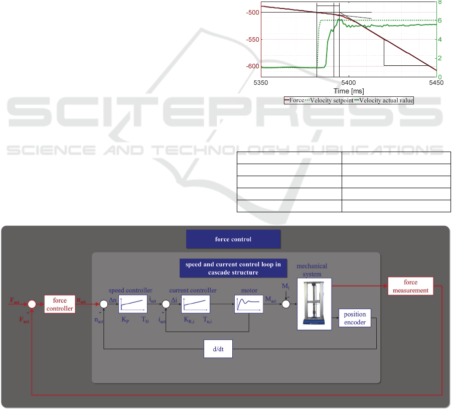
difference is transferred to the velocity controller as
a speed set point via the force controller. This offers
another advantage. In order to be able to specify the
speed set point, either a corresponding variable can
be applied in the control loop or the IEC 61131-3-
compliant motion control (MC) commands are used.
The MC blocks are available in a library and are
instantiated in the programs. The parameters are set
in the state machine. The MC_MoveVelocity was
utilized in detail, which gives a speed set point via
the NC axis technology object to the servo inverter
and thus the velocity controller. This results in the
structure for force control as illustrated in Figure 5.
4.2 Experiments and Parameterization
With regard to the design of a force control on
electromechanical feed axes, no generally applicable
regulations are known yet. For this reason, manual
parameterization is carried out first. When
controlling process forces, the process itself is part
of the controlled system. Accordingly, the control
plant of the force controller consists of the
subordinate velocity and current control loop, as
well as the mechanics of the axis and the process. In
order to simulate a process or a resulting process
force, a flexible spring element with a linear
characteristic was selected. In this way, a load with
high reproducibility can be initiated with a
movement of the axis against the resistance. A P-
controller was initially selected as the controller
type. This is justified by the fact that P-controllers
can be designed quickly and easily with just one
parameter. Moreover, the fact that the controlled
system or the process already contains an integrating
part can be exploited. Furthermore, it makes sense to
integrate an actual value filter in the control loop in
order to reduce the measurement noise and improve
the signal quality. A moving average filter with a
time window of 10 ms was selected for this purpose.
In addition, it should be investigated to what
extent general setting regulations from the time
range can be used for the design of the force control.
Hence, it is necessary to carry out an identification
of the control plant, which includes the process or
the flexible spring, respectively. During
identification, a stepwise excitation of 5 mm/s is
activated at the input of the velocity control loop. A
speed offset of 1 mm/s was determined in order to
avoid static friction effects. The force is recorded at
the output of the control plant. The result of the
identification and the relevant parameters are shown
in Figure 6 and summarized in Table 2.
Figure 6: Identification of the controlled system.
Table 2: Controlled system parameters.
Time difference
dt = 26 ms
Force difference
dF = 50 N
Actual velocity
v
av
= 5,5 mm/s
Dead time
T
d
= 10 ms
Delaying time
T
u
= 2,8 ms
Figure 5: Force control structure.
Force [N]
Velocit
y
[mm/s]
T
d
=10ms T
u
=2,8ms
dF=50N
dt=26ms
Performance Analysis of the Force Control for an Electromechanical Feed Axis with Industrial Motion Control
671

The controlled system has an IT1 behavior and the
gain can be calculated according to the following
equation:
K
SI
= dF / (dt * v
av
) (3
)
Based on the determined values, K
SI
is
350 N/mm. The gain factor for the force controller
can be calculated on the basis of these characteristic
values. For this purpose, Samal´s setting instruction
(Lunze, 2005):
K
P
= π / (4*K
SI
* (T
d
+ T
u
)) (4
)
and the calculation of the symmetrical optimum
according to (Lutz and Wendt, 1995):
K
P
= 1 / (a*K
SI
* (T
d
+ T
u
)) (5
)
were selected. Here, the parameter a is a damping
factor that has been set to the value 2. The calculated
parameters are summarized in Table 2.
Table 2: Parameters for the force control.
adjustment rule Parameter
Samal K
P
= 175 *10
-3
[mm/Ns]
Symmetrical Optimum K
P
= 112 *10
-3
[mm/Ns]
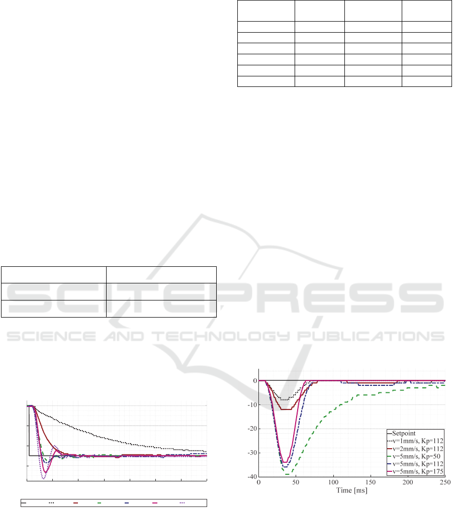
To assess the controller behavior, a preload of
500 N was first generated and subsequently a force
jump of 50 N was specified for the closed control
loop. The step responses for the different
amplification factors with the unit [
10
-3
mm/Ns] are
shown in Figure 7.
Figure 7: Step response of the controllers.
The controller performance is assessed on the
basis of comparison criteria in the time domain. The
rise and set time as well as the overshoot were
selected as criteria. A tolerance band of ± 2 N was
defined for this. The characteristic values for the
different parameterizations are compared in Table 3.
Table 3: Comparison criteria in the time domain.
K
P
[10
-3
m/Ns]
Rise time
[ms]
Set time
[ms]
Overshoot
[N]
10 721 721 -
50 177 177 -
100 57 132 5
112 49 89 7
150 46 120 17
175 37 121 23
In Figure 7 it can already be clearly seen that the
rise time becomes smaller with increasing
amplification factor. However, the overshoot range
is also increasing. With sufficiently small
amplification factor, no overshoot occurs. Moreover,
dead time of 15 ms was identified for the system.
Finally the adjustment rule based on the symmetrical
optimum offers a good compromise between
overshoot height and rise time.
Another interesting aspect to investigate is the
system behavior in the case of contact. The start of
the process should be recognized automatically
based on the threshold force of 1,5 N and trigger the
switch from position control to force control. A
constant velocity was specified in order to cause a
contact situation and to simulate an disturbing
process force. The setpoint of the force is 0 N, so
that the disturbance caused by the contact is
corrected. For this, the parameterization according to
the symmetrical optimum was first selected and the
behavior at different velocities was considered. The
gain factor was then varied at a velocity of 5 mm/s.
The results are illustrated in Figure 8.
Figure 8: System behavior in case of contact.
Due to the dead time during the switchover, the
starting velocity has the greatest influence on the
height of the acting force. The amplification factor
has an influence, too. The greater the amplification
factor is chosen, the smaller is the force. However,
this influence is marginal compared to the impact of
the starting velocity. On the other hand, the gain
factor has major impact on the settling time. The
0 100 200 300 400 500 600 700
Time [ms]
-560
-540
-520
-500
Force [N]
Setpoint Kp=10 Kp=50 Kp=100 Kp=112 Kp=150 Kp=175
Force [N]
ICINCO 2020 - 17th International Conference on Informatics in Control, Automation and Robotics
672

higher the factor is selected, the faster the
disturbance can be corrected. At some point a
saturation effect occurs here. There is only a slight
difference between adjustment instruction
accordingly Samal and the symmetrical optimum. A
further increase in the gain would therefore only
have a minor effect.
By switching from the position control, it is
possible to specify a force profile. It is important to
examine how well the controller follows the set
point. For the experiment, a positioning ramp is
initially specified, which is replaced by a set point
force curve at a threshold of 500 N. A force increase
of 100 N/s up to a force of 1000 N was specified
here. The system behavior of different parameter
settings is shown in Figure 9.
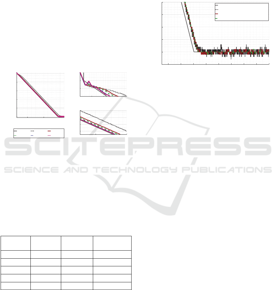
Figure 9: System behavior for a defined force curve.
Due to the dead time when switching, the
starting velocity is initially maintained. The force
control reacts after the dead time of 15 ms. With
bigger gain factors, there is then a slight overshoot
(see Figure 9, up right). However, the contouring
error is significantly smaller here (see Figure 9,
down right). These values are summarized in
Table 4.
Table 4: Comparison Criteria of the force ramp.
K
P
Overshoot
Contouring
error
Delay time
10 - 27 N 270 ms
30 - 10 N 84 ms
50 - 5 N 51 ms
112 3 N 2 N 21 ms
175 4 N 2 N 15 ms
Here, the difference between the adjustment
instruction accordingly Samal and the symmetrical
optimum is also only marginal. Overall, the
adjustment rule of the symmetrical optimum is a
suitable criterion for the parameterization of the
force controller for this use case.
Moreover, the effect of the actual value filter
setting on the control was also examined. Different
filter time windows for the gain factor of the
symmetrical optimum were compared. Here, the
force curve was specified again. The results are
shown and summarized in Figure 10.
Figure 10: Influence of the force actual value filter.
It can be seen that a significant reduction in
measurement noise can be achieved with the length
of the sliding window. The variance of the measured
value decreases with increasing length and
satisfactory results are achieved at 10 ms.
5 CONCLUSION
In this publication, the combination of force control
with position control was presented for an
electromechanical axis. The focus of the
investigations was on the controller performance.
Empirical setting factors and general adjustment
rules were evaluated with regard to their suitability.
It has been found here that good results can be
achieved with the symmetrical optimum. It was also
shown that the functionality of the switchover is
given. Moreover, the force is quickly adjusted in the
case of contact. In addition, the control follows
specified force profiles with a small contouring
error. If necessary, this can be reduced even further
with a feedforward control.
The external PC was initially used for
commissioning and implementation. The
performance was assessed for this system structure.
A system expansion with a top-hat rail industrial PC
is perspective possible and also envisaged. It can be
integrated directly via the backplane bus. This
requires porting the project to the IPC. In this way,
the communication dead times due to the EtherCAT
connection are eliminated and a further
improvement in performance can be expected. The
implementation of the corresponding measures is
2000 4000 6000
Time [ms]
-1000
-900
-800
-700
-600
-500
Force [N]
Setpoint Kp=10 Kp=30
Kp=50 Kp=112 Kp=175
700 800 900 1000 1100
Time [ms]
-520
-510
-500
-49
0
Force [N]
3800 4000 4200 4400
Time
[
ms
]
-840
-820
-800
-780
Force [N]
4600 4800 5000 5200 5400 5600 5800 6000 6200
Time
[
ms
]
-1005
-1000
-995
-990
-985
-980
Force [N]
Setpoint
Filter 1ms (Variance = 0.7139)
Filter 5ms (Variance = 0.1699)
Filter 10ms (Variance = 0.1006)
Performance Analysis of the Force Control for an Electromechanical Feed Axis with Industrial Motion Control
673

planned in future studies. The potential of complex
control algorithms should also be considered there.
ACKNOWLEDGEMENTS
Funded by the European Union (European Social
Fund) and the Free State of Saxony.
REFERENCES
Schröder, D., 2001. Elektrische Antriebe – Regelung von
Antriebssystemen, Springer Verlag Berlin, 2
nd
edition.
Allwood, J. M., et al., 2016. Closed-loop control of
product properties in metal forming. In CIRP Annals –
Manufacturing Technology, 65, 573-596.
Ulsoy, A.G. and Koren, Y., 1993. Control of Machining
Process. In Journal of Dynamic Systems Measurement
and Control, 115, 301-308.
Ulsoy, A.G. and Koren, Y., 1989. Applications of adaptive
control to machine tool process control. In IEEE
Control Systems Magazine, 9(4), 33-37.
Koren, Y. and Masory, O., 1981, Adaptive Control with
Process Estimation. In CIRP Annals, 30(1), 373-376.
Ulsoy, A.G., Koren, Y. and Rasmussen, F., 1983.
Principal developments in the adaptive control of
machine tools. In Journal of Dynamic Systems,
Measurement, and Control, 105(2), 107-112.
Liu, Y., Cheng, T. and Zuo, L., 2001. Adaptive control
constraint of machining processes. In The
International Journal of Advanced Manufacturing
Technology, 17(10), 720-726.
Landers, R.G., Ulsoy, A.G. and Ma, Y.-H., 2004. A
comparison of model based machining force control
approaches. In International Journal of Machine Tools
and Manufacture, 44(7–8), 733-748.
Zuperl, U., Cus, F. and Milfelner, M., 2005, Fuzzy Control
Strategy for an Adaptive Force Control in End-
Milling, In Journal of Materials Technology, 164-165,
1472-1478.
Xu C. and Shin Y.C., 2008. An adaptive fuzzy controller
for constant cutting force in end-milling processes. In
Journal of Manufacturing Science and Engineering,
130 (3).
Kim, D. and Jeon, D., 2011. Fuzzy-logic control of cutting
forces in CNC milling processes using motor currents
as indirect force sensors. In Precision Eng., 35(1),
143-152.
Haber, R.E. and Alique, J.R., 2004. Nonlinear internal
model control using neural networks: an application
for machining processes. In Neural Computing &
Applications, 13, 47–55.
Yao, X., et al., 2013. Machining force control with
intelligent compensation. In International Journal of
Advanced Manufacturing Technology, 69, 1701–1715.
Stemmler, S., et al., 2017. Model Predictive Control for
Force Control in Milling. In IFAC-PapersOnLine,
50(1), 15871-15876.
Posdzich, M., et al., 2019. Burnishing of prismatic
workpieces on three-axis machine enabled by closed
loop force control. In 52nd CIRP Conference on
Manufacturing Systems (CMS), 81, 1028-1033.
Zirn, O., 2008. Machine Tool Analysis – Modelling,
Simulation and Control of Machine Tool
Manipulators. Habilitation, ETH Zürich.
Lunze, J., 2005. Regelungstechnik 1: Systemtheoretische
Grundlagen, Analyse und Entwurf einschleifiger
Regelungen, Springer Vieweg. Heidelberg, 5
th
edition.
Lutz, H. and Wendt, W., 1995. Taschenbuch der
Regelungstechnik, Harri Deutsch. Frankfurt, 1
st
edition.
ICINCO 2020 - 17th International Conference on Informatics in Control, Automation and Robotics
674