Frank, T., Wielitzka, M., Dagen, M. and Ortmaier, T.
Reduced-order Modeling of Parameter Variations for Parameter Identification in Rubber Curing.
DOI: 10.5220/0009865106590666
In Proceedings of the 17th International Conference on Informatics in Control, Automation and Robotics (ICINCO 2020), pages 659-666
ISBN: 978-989-758-442-8
Copyright
c
 2020 by SCITEPRESS – Science and Technology Publications, Lda. All rights reserved
659

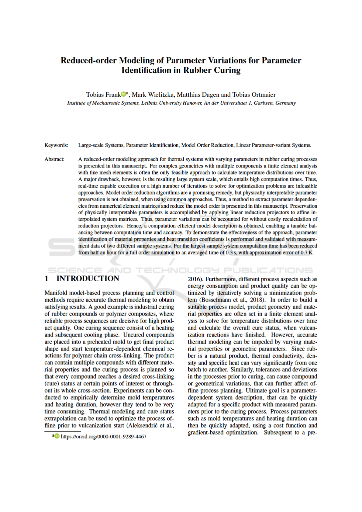
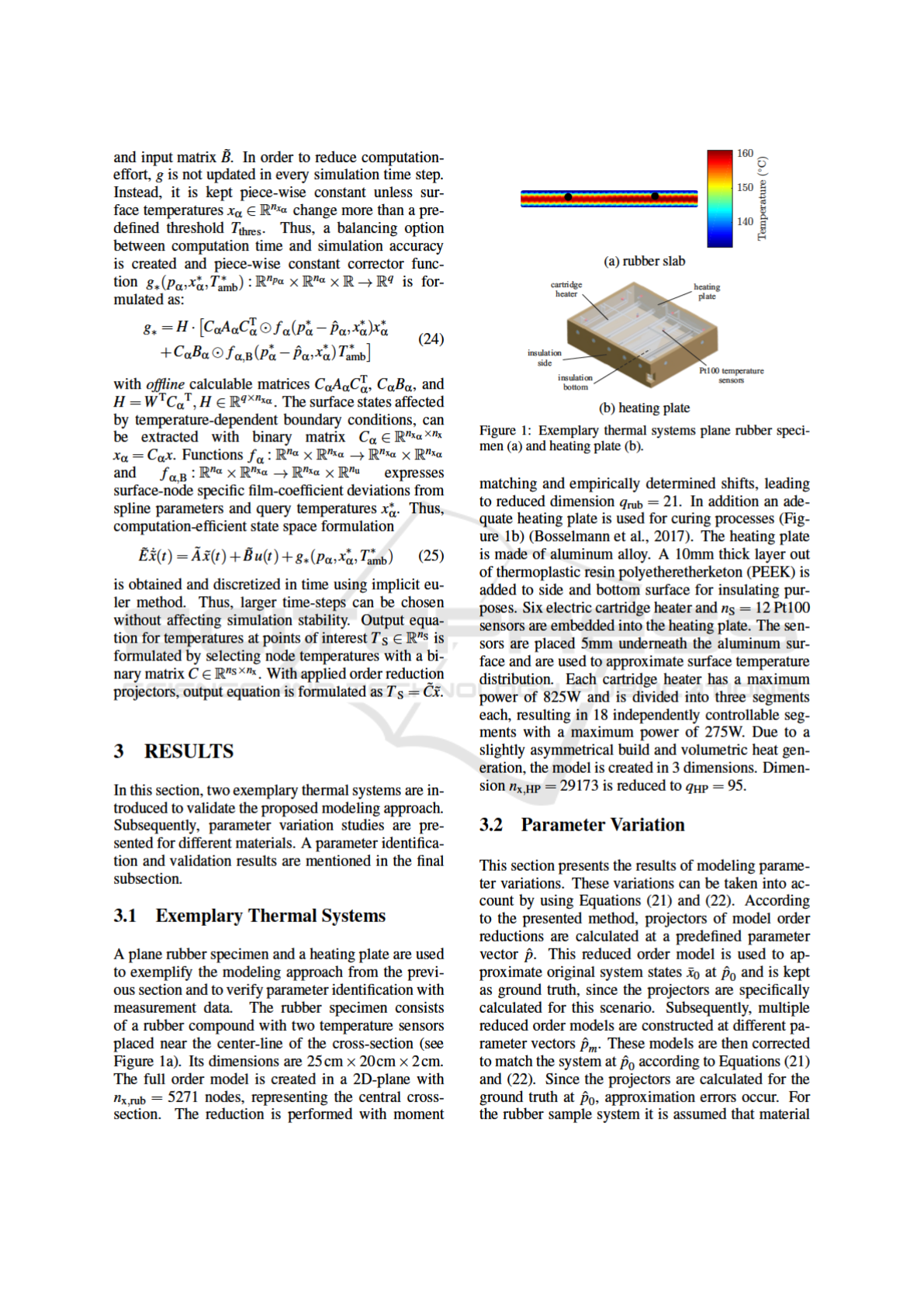
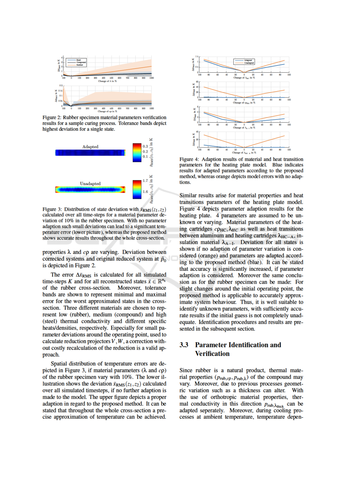
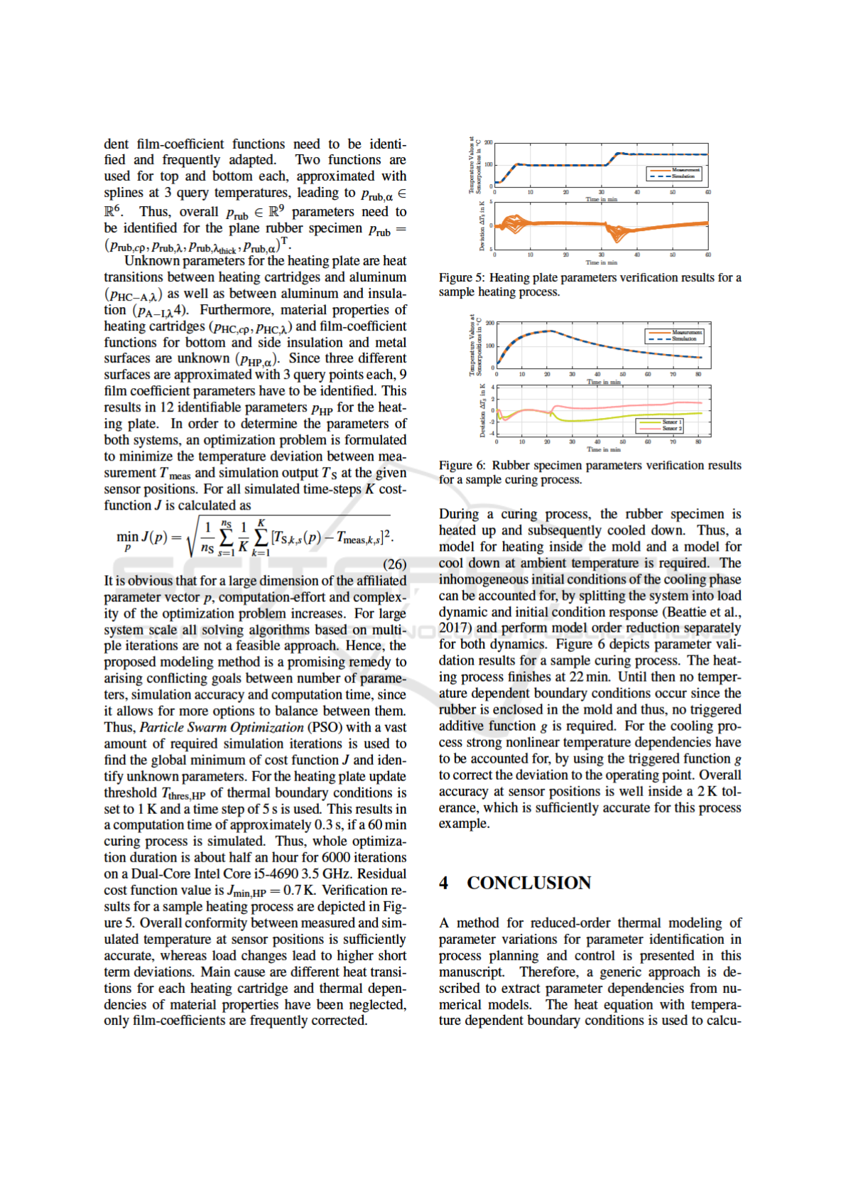
cise process planning, determined process parameters
have to be maintained online. Industrial heating sys-
tems such as molds need to be controlled properly
to ensure a desired temperature distribution at con-
tact surfaces or product interfaces (Wang et al., 2015).
Model-based control approaches are favourable, since
multiple process criteria and limitations can be ac-
counted for. However, unknown or temperature de-
pendent boundary conditions to the ambient can lead
to disturbances or model errors. Furthermore, it is
beneficial to identify mold material properties, ther-
mal resistances and heat transitions, due to material
contact surfaces or components with unknown assem-
bly. Thus, a computation-efficient and parameter-
dependent system description is required, to enable
real-time computation for model-based control and
state estimation or to perform high amounts of itera-
tions in short time to solve for optimization problems.
Besides curing processes, multiple approaches
have been introduced to incorporate thermal models
in process control approaches. If applicable, model
simplifications, such as reduction of spatial dimen-
sion, using symmetry or neglecting complex geomet-
ric structures, are an easy and well used remedy. Spe-
icher et al. (Speicher et al., 2014) used a lower spatial
dimension model to reduce computation complexity
and estimate plate temperatures in a hot rolling pro-
cess. Furthermore, linearizations are applicable, if
the system maintains in a specific operating area. In
this case linear model order reduction can be a pow-
erful tool to lower system scale (Yuan et al., 2017),
(Benner et al., 2019). If these simplifications are
improper, parametric model order reduction methods
to approximate large scale systems can be used, but
yield possible limitations in number of accountable
parameters, online adaption and reduced system or-
der (Benner et al., 2015). A proper choice to reduce
the model would be Proper Orthogonal Decomposi-
tion (POD) (Astrid, 2004). This approach for nonlin-
ear systems is especially effective with the use of dis-
crete empirical interpolation (DEIM) (Chaturantabut
and Sorensen, 2010). However, sample trajectories
(snapshots) of already validated full order models or a
high amount of measurement data are required, when
a vast amount of varying parameters occur. Sun et al.
used balancing and POD to model parameter uncer-
tainties by lumping parameters into the input vector
and incorporate them into the reduction process (Sun
and Hahn, 2006).
In this work a novel method for thermal modeling
with accountable parameter variations is proposed.
The system description can be directly derived from
finite element analysis. Main achievements are for-
mulation of thermal linear parameter-variant (LPV)
systems from nonlinear partial differential equations,
model order reduction of LPV systems, and parameter
preservation to enable optimization and identification
procedures. Furthermore, state-dependent parameter
changes as caused temperature-dependent boundary
conditions can be accounted for during simulation,
enabling a balancing between computation time and
accuracy.
2 METHODS
In this section a thermal modeling approach is
described in order to achieve a linear parameter-
dependent system description from numerical ele-
ment matrices of a FEA. Subsequently, model order
reduction of the LPV system and parameter preser-
vation is explained. Ultimately, a computation effi-
cient system description with approximated temper-
ature dependent boundary conditions is gained and
used for results in Section 3.
2.1 Thermal Modeling
The spatial-temporal dependent temperature distribu-
tion T (z, t) of a distributed parameter system within
domain Ω ⊂ R
n
dim
, ∀z = (z
1
, . . . , z
n
dim
)
T
∈ Ω at time
t ∈ R
+
and dimension n
dim
∈ {1, 2, 3} can be de-
scribed as a scalar field with parabolic partial differen-
tial heat equations (PDEs) and Fourier’s law, leading
to infinite dimensional equation:
c(z)ρ(z)
∂T (z, t)
∂t
= div(Λ(z)∇T (z, t)) + ω(z, t). (1)
The ∇-operator denotes partial derivatives with re-
spect to z. Internal heat sources are expressed as ω
in [Wm
−3
]. Material properties c and ρ are specific
heat and density. Λ denotes the thermal conductivity
tensor which can account for anisotropic heat conduc-
tion. The following three assumptions are made for
the material coefficients:
Assumption 1. All material properties c(z), ρ(z),
and Λ(z) are time and state invariant.
Assumption 2. System domain Ω consists of
multiple components Ω
j
, Ω =
.
S
j∈{1,...,n
comp
}
Ω
j
,
j ∈ {1, . . . , n
comp
}, n
comp
∈ N
+
made of homo-
geneously distributed materials with properties
c(z
j
) · ρ(z
j
) = (cρ)
j
and Λ(z
j
) = Λ
j
, ∀z
j
∈ Ω
j
.
Assumption 3. Thermal conductivity tensor Λ
j
can
either be reduced to a scalar value λ
j
for isotropic
ICINCO 2020 - 17th International Conference on Informatics in Control, Automation and Robotics
660

conduction throughout a system component or is as-
sumed to be a diagonal matrix with orthotropic prop-
erties Λ
j
= diag(λ
j,z
1
, . . . , λ
j,z
n
dim
).
The initial condition T (z, 0) = T
0
(z), z ∈ Ω sets an
inhomogenous temperature distribution T
0
through-
out the domain. Furthermore, heat transfer between
surface and surrounding fluid or gas also known as
Robin boundary conditions φ
R
have to be accounted
for. This boundary condition is formulated as su-
perimposed heat flux phi
R
= φ
conv
+ φ
rad
caused by
heat emission φ
rad
and convection φ
conv
with defined
on z
B
∈ ∂Ω as:
φ
conv
(z
B
, t) = α(T (z
B
, t), z
B
)(T (z
B
, t) − T
amb
), (2)
φ
rad
(z
B
, t) = ε(z
B
)σ

T (z
B
, t)
4
− T
4
amb

. (3)
Herein, z
B
corresponds to coordinates of domain sur-
face ∂Ω exposed to ambient. Convective heat flux
φ
conv
is calculated from temperature difference be-
tween surface and ambient temperature T
amb
, multi-
plied with temperature and geometric dependent film
coefficient α(T (z
B
, t), z
B
). Radiative heat flux φ
rad
is nonlinear in temperature and can be computed by
Stefan-Boltzmann-law with emission coefficient ε(z
B
)
and Stefan-Boltzmann constant σ. Thus, a nonlinear
partial differential equation:
∂
∂t
T (z, t) = f (T (z, t), T
amb
) (4)
needs to be solved for T (z, t). However, nonlin-
ear equation (4) can be transformed into a linear
parameter-variant (LPV) system description, if non-
linear dependencies are moved into system coeffi-
cients (Bruzelius, 2004). This is applicable for ther-
mal systems. Thus, Robin boundary conditions are set
to
φ
R
(z
B
, T ) = α
tot
(T (z
B
), z
B
)(T (z
B
) − T
amb
), (5)
with total film coefficient:
α
tot
(T (z
B
, t), z
B
) = α(T (z
B
, t), z
B
) +
φ
rad
(z
B
, t)
T (z
B
, t) − T
amb
. (6)
Nevertheless, α
tot
(T (z
B
, t), z
B
) still depends on local
geometry and hence, is a function of z
B
. However, it
can be assumed as a surface area specific function:
Assumption 4. Superimposed film coefficient
function α
tot
(T (z
B
, t), z
B
) is spatially inde-
pendent throughout specific surface areas
∂Ω
i
⊂ ∂Ω, i ∈ {1, .., n
surf
} ⊂ N
+
, leading to discrete
α
tot
(T (z
B,i
, t), z
B,i
) = α
tot,i
(T (z
B,i
, t)), ∀z
B,i
∈ ∂Ω
i
.
According to (Frank et al., 2019) area-specific
film-coefficient functions are approximated by shape-
preserving piece-wise cubic interpolation at prede-
fined query points. Thus, identifiable parameters
p
α
are created to parametrize temperature dependent
boundary conditions. Moreover, p
cρ
∈ R
n
comp
and
p
λ
∈ R
n
comp
n
dim
describe material properties. Com-
bined parameter vector p ∈ P ⊆ R
n
p
contains all of
the variant system parameters. Domain Ω is spa-
tially discretized using weak formulation and finite
element method to get a lumped element model. This
results in a system of linear-parameter variant ordi-
nary differential equations (ODEs) (Huang and Us-
mani, 1994),(Li and Qi, 2010). First order shape
functions f
T
s
(z) : x(t) 7→ T (z, t) are used to map node
temperatures x ∈ R
n
x
of finite element mesh to con-
tinuous temperature distribution T (z, t). Eventually,
following system description is obtained and can be
exported from finite element analysis, but only at a
specific operating point with constant parameters ˆp,
E|
ˆp
cρ
˙x = A|
ˆp
α
, ˆp
λ
x + B|
ˆp
α
u, (7)
with damping matrix E ∈ R
n
x
×n
x
, conductivity matrix
A ∈ R
n
x
×n
x
, load matrix B ∈ R
n
x
×n
u
, and input vec-
tor u ∈ R
n
u
. All of the matrices are in numeric form,
but accessible parameters are required. Thus, a form
of affine parameter dependence is formulated for the
matrices similar to (Feng et al., 2016). In regard to
assumptions 1 and 2, matrices are specified as:
E(p
cρ
) ≈ E
0
+
n
comp
∑
j=1
E
cρ, j
· p
cρ, j
,
(8)
A(p
α
, p
λ
, x) ≈ A
0
+ A
α
 P
A,α
(x)
+
n
comp
∑
j=1
n
dim
∑
k=1
A
λ,k, j
· p
λ,k, j
,
(9)
B(p
α
) ≈ B
0
+ B
α
 P
B,α
(x).
(10)
Component-specific matrices E
cρ, j
and A
λ,k, j
are mul-
tiplied with the corresponding material properties. In
the equations above n
comp
describes the components
with varying parameters. Parameter that are already
known or of less significance can be considered by E
0
and A
0
. These matrices are extracted from linearized
numerical matrices by setting the varying parameters
near zero. E
cρ, j
and A
λ,k, j
are formulated according
to the following component-wise ( j) matrix export
E
0
= E|
( ˆp
cρ
→0)
, (11)
E
cρ, j
= E|
( ˆp
cρ, j
=1)
− E
0
, (12)
A
0
= A|
(
ˆ
P
λ
→0, ˆp
α
→0)
, (13)
A
λ,k, j
= A|
( ˆp
λ,k, j
=1, ˆp
α
→0)
− A
0
, (14)
B
0
= B|
( ˆp
α
→0)
, (15)
A
α
=
n
surf
∑
i=1
A|
(
ˆ
P
λ
→0, ˆp
α,i
=1)
− A
0
, (16)
B
α
=
n
surf
∑
i=1
B|
( ˆp
α,i
=1)
− B
0
. (17)
Reduced-order Modeling of Parameter Variations for Parameter Identification in Rubber Curing
661

Matrices P
A,α
(x) ∈ R
n
x
×n
x
and P
B,α
(x) ∈ R
n
x
×n
u
are
multiplied to corresponding differential matrices with
element-wise Hadamard product  and contain
state(node)-specific film-coefficients. Every matrix
entry represents a node, that is assigned to a compo-
nent or surface. Thus, parameters p
α
, including spline
approximation parameters, can be used to construct
P
A,α
(x) and P
B,α
(x). These matrices are state depen-
dent, because thermal boundary conditions vary with
temperature. Eventually, a LPV description derived
from numerical FEA is generated including physi-
cally interpretable parameters
E(p
cρ
) ˙x = A(p
α
, p
λ
, x)x + B(p
α
, x)u. (18)
2.2 Model Order Reduction
System descriptions derived from FEA tend to have
large scale, especially if complex geometries or
multiple components are present. Thus, computation-
costs are very high and prevent real-time capable
execution or high amount of simulation iterations
for optimization problems. If model simplifications,
symmetry or reduction in spatial dimensions are
infeasible, model order reduction methods can be
powerful tools, to further reduce computation time
with sufficiently accurate simulation results. How-
ever, most approaches are only valid for linear system
descriptions. Moreover, physical interpretation of
reduced systems and parameter access is no longer
possible, since the reduced states do not represent
temperatures. Hence, already validated full order
models are required and have to be linearized at an
operating point. Parametric model order reduction
methods are used as a remedy, but are limited to
constant parameters or further extend reduced system
descriptions. Data-based methods are based on
system snapshots, which can be difficult to obtain,
if no measurement data can be acquired or multiple
time-consuming simulations of a full order model
have to be performed. A promising remedy has
been introduced in (Frank et al., 2018), where
system description (18) is split into a linearized
part and an additive function to correct operating
point deviations. Classical model order reduction
for linear systems is used to calculate projectors,
that are also applied to the corrective function. A
similar approach is used in this work, as model order
reduction is calculated for a linearized system and
parameter variation are added subsequently. Thus,
time consuming reduction algorithms are performed
only once, and parameter variations or state de-
pendent changes can be accounted for separately.
For applying projection-based model reduction, an
arbitrary operating point ˆp can be inserted in equation
(18) to obtain a linear system (7), without repeated
export of numerical matrices from FEA. Model
order reduction using Rational Krylov projections
(Grimme, 1997) has been found to be most robust
in approximating system behaviour with subsequent
deviations form chosen operating point. In this
method moments of the original transfer function
are approximated at predefined frequency shifts,
so that as many moments as possible are matched
between original and reduced order system. Even-
tually, linear projectors W ∈ R
n
x
×q
and V ∈ R
n
x
×q
are obtained from applied model order reduction
with reduced dimension q  n. Hence, reduced
matrices
˜
A|
ˆp
α
, ˆp
λ
= W
T
A|
ˆp
α
, ˆp
λ
V ,
˜
A|
ˆp
α
, ˆp
λ
∈ R
q×q
,
˜
B|
ˆp
α
= W
T
B|
ˆp
α
,
˜
B|
ˆp
α
∈ R
q×n
u
,
˜
E|
ˆp
cρ
= W
T
E|
ˆp
cρ
V ,
E|
ˆp
cρ
∈ R
q×q
, and projected state vector ˜x ∈ R
q
can
be calculated. Transformation between state-vectors
can be expressed as:
˜x = W
T
x, x ≈ ¯x = V ˜x, (19)
with approximated full order state vector ¯x ∈ R
n
x
. Re-
duced system description at operating point ˆp
˜
E|
ˆp
cρ
˙
˜x =
˜
A|
ˆp
α
, ˆp
λ
˜x +
˜
B|
ˆp
α
u (20)
is extended to consider material uncertainties, using
affine characteristics of equations (8) and (9). Thus,
damping and system matrix are obtained from:
˜
E =
˜
E|
ˆp
cρ
+W
T

n
comp
∑
j=1
E
cρ, j
· (p
cρ, j
− ˆp
cρ, j
)

V ,
(21)
˜
A =
˜
A|
ˆp
α
, ˆp
λ
+W
T

n
comp
∑
j=1
n
dim
∑
k=1
A
λ,k, j
· (p
λ,k, j
− ˆp
λ,k, j
)

V ,
(22)
˜
B =
˜
B|
ˆp
α
.
(23)
Since, projectors are applied although approximated
transfer function of the original system varies, appli-
cability of introduced transformations has to be inves-
tigated. It is obvious that amount of material prop-
erties and deviation is limiting overall approxima-
tion quality. For thermal systems with rather slug-
gish system dynamic, a variation of damping pa-
rameters is not as crucial as a variation of thermal
conductivity, especially if transfer function moments
at lower frequency shifts are approximated. De-
tailed results are presented in section 3. For identi-
fication purposes or process planning, these changes
can be made before the simulation is started. How-
ever, state dependent change of boundary condi-
tions have to be accounted for during the computa-
tion. Thus, online correction of film-coefficients in-
troduced in (Frank et al., 2018) is used. Therefore,
additionally to previous equations, a non-constant
state-dependent term g is added to system matrix
˜
A
ICINCO 2020 - 17th International Conference on Informatics in Control, Automation and Robotics
662

Reduced-order Modeling of Parameter Variations for Parameter Identification in Rubber Curing
663

ICINCO 2020 - 17th International Conference on Informatics in Control, Automation and Robotics
664

Reduced-order Modeling of Parameter Variations for Parameter Identification in Rubber Curing
665

late temperature distributions over time in 2 or 3 di-
mensional problems. Since large system scales can
arise from finite element analysis, model order re-
duction is applied to reduce computation time. This
computation-efficient description is required for solv-
ing optimization problems with a high amount of iter-
ations or meeting real-time demands. However, basic
model order reduction methods are only valid for lin-
ear models. If the system can not be linearized prop-
erly, temperature dependent boundary conditions as
well as parameter uncertainties have to be accounted
for. Parametric reduction algorithms are either based
on system snapshots or entail higher reduced orders
and larger projection matrices. Thus, a method to pre-
serve physically interpretable parameters, while using
rational Krylov model order reduction algorithms is
proposed. This is especially applicable for small vari-
ations around a well defined initial operating point.
Hence, neither a validation of the full order model be-
fore formulating the reduced model is required nor
many time consuming experiments to get measure-
ment data. Instead system parameters are identi-
fied and validated with a reduced system formulation.
Moreover, temperature dependencies during the pro-
cess can be modeled and a parameterizable balancing
between computation time and accuracy is possible.
Thus, online process adaptions according to (stochas-
tic) parameter variations are possible without costly
recalculation of model order reduction. The approach
is demonstrated for two sample systems, which mate-
rial and heat transition parameters are identified with
reduced-order models. Therefore, particle swarm op-
timization can be used to find the global minimum of
a formulated cost-function. Moreover, computation
times are within real-time restrictions and thus, pre-
sented models are used for model-based temperature
control, process predictions and state estimation.
REFERENCES
Aleksendri
´
c, D., Carlone, P., and
´
Cirovi
´
c, V. (2016). Op-
timization of the temperature-time curve for the cur-
ing process of thermoset matrix composites. Applied
Composite Materials, 23(5):1047–1063.
Astrid, P. (2004). Reduction of process simulation models
: a proper orthogonal decomposition approach. PhD
thesis, Department of Electrical Engineering.
Beattie, C., Gugercin, S., and Mehrmann, V. (2017). Model
reduction for systems with inhomogeneous initial con-
ditions. Systems & Control Letters, 99:99 – 106.
Benner, P., Gugercin, S., and Willcox, K. (2015). A
survey of projection-based model reduction methods
for parametric dynamical systems. SIAM Review,
57(4):483–531.
Benner, P., Herzog, R., Lang, N., Riedel, I., and Saak, J.
(2019). Comparison of model order reduction meth-
ods for optimal sensor placement for thermo-elastic
models. Engineering Optimization, 51(3):465–483.
Bosselmann, S., Frank, T., Wielitzka, M., Dagen, M., and
Ortmaier, T. (2017). Thermal modeling and decen-
tralized control of mold temperature for a vulcaniza-
tion test bench. In 2017 IEEE Conference on Control
Technology and Applications (CCTA), pages 377–382.
Bosselmann, S., Frank, T., Wielitzka, M., and Ortmaier, T.
(2018). Optimization of process parameters for rub-
ber curing in relation to vulcanization requirements
and energy consumption. In 2018 IEEE/ASME Inter-
national Conference on Advanced Intelligent Mecha-
tronics (AIM), pages 804–809.
Bruzelius, F. (2004). Linear parameter-varying systems: An
approach to gain scheduling: Zugl.: Goteborg, Univ.,
Diss., 2004. PhD thesis, School of Electrical Engi-
neering.
Chaturantabut, S. and Sorensen, D. C. (2010). Nonlinear
model reduction via discrete empirical interpolation.
SIAM Journal on Scientific Computing, 32(5):2737–
2764.
Feng, L., Yue, Y., Banagaaya, N., Meuris, P., Schoenmaker,
W., and Benner, P. (2016). Parametric modeling and
model order reduction for (electro-)thermal analysis
of nanoelectronic structures. Journal of Mathematics
in Industry, 6(1):10.
Frank, T., Bosselmann, S., Wielitzka, M., and Ortmaier, T.
(2018). Computation-efficient simulation of nonlinear
thermal boundary conditions for large-scale models.
IEEE Control Systems Letters, 2(3):351–356.
Frank, T., Wieting, S., Wielitzka, M., Bosselmann, S., and
Ortmaier, T. (2019). Identification of temperature-
dependent boundary conditions using mor. Interna-
tional Journal of Numerical Methods for Heat & Fluid
Flow, ahead-of-print.
Grimme, E. (1997). Krylov Projection Methods for Model
Reduction. PhD thesis, Department of Electrical and
Computer Engineering.
Huang, H.-C. and Usmani, A. S. (1994). Finite Element
Analysis for Heat Transfer. Springer London, London.
Li, H.-X. and Qi, C. (2010). Modeling of distributed pa-
rameter systems for applications - a synthesized re-
view from time & space separation. Journal of Pro-
cess Control, 20(8):891 – 901.
Speicher, K., Steinboeck, A., Kugi, A., Wild, D., and
Kiefer, T. (2014). Analysis and design of an extended
kalman filter for the plate temperature in heavy plate
rolling. Journal of Process Control, 24(9):1371 –
1381.
Sun, C. and Hahn, J. (2006). Model reduction in the pres-
ence of uncertainty in model parameters. Journal of
Process Control, 16(6):645 – 649.
Wang, D.-h., Dong, Q., and Jia, Y.-x. (2015). Mathemat-
ical modelling and numerical simulation of the non-
isothermal in-mold vulcanization of natural rubber.
Chinese Journal of Polymer Science, 33(3):395–403.
Yuan, C. D., Rudnyi, E. B., Baumgartl, H., and Bechtold,
T. (2017). Model order reduction and system simula-
tion of a machine tool for real-time compensation of
thermally induced deformations. In 2017 IEEE Inter-
national Conference on Advanced Intelligent Mecha-
tronics (AIM), pages 1071–1076.
ICINCO 2020 - 17th International Conference on Informatics in Control, Automation and Robotics
666