Robustness Estimation of Large Deviations in Linear Discrete-time
Systems with Control Signal Delay
Nina Vunder
1 a
and Natalia Dudarenko
2 b
1
Institute of Control Engineering, TU Braunschweig, Hans-Sommer-Str. 66, Braunschweig, Germany
2
Department of Control Systems and Industrial Robotics, ITMO University, 49 Kronverksky Pr., Saint-Petersburg, Russia
Keywords:
Discrete-time System, Delay, Large Deviations, Peak Effect, Sensitivity Analysis.
Abstract:
The article deals with robustness estimation of large deviations in free motion of linear discrete-time systems
to parameter variations of the state matrix. A tracking discrete-time system with the modal control law is
considered in the paper. The modal control law is designed taking into account the value of delay and the
deviation. It is assumed that parameters of the system are linearly dependent on the uncertainties. The problem
is solved with the state space approach and the sensitivity theory methods. An upper bound estimation of
trajectory deviations for discrete-time systems is obtained. The estimation contains the condition number of
the eigenvectors matrix of the system state matrix. Therefore, sensitivity functions of singular values of the
eigenvectors matrix are used to calculate the robustness estimation of the deviations. Based on the obtained
equations, an algorithm for the robustness estimation of large deviations in linear discrete-time systems with
parametric uncertainties is proposed. Two cases of control signal delay are considered in the paper. The first
case relates to predictable delay of control signal, and the second one relates to unpredictable delay of control
signal. The results are supported with an examples.
1 INTRODUCTION
Large deviations (peak effects) in the free motion of a
linear system occur due to nonzero initial conditions
in the absence of exogenous input signal. The large
deviation problem has been investigated by special-
ists in control theory and signal processing for a long
time. Firstly, the relationship between system poles
and large deviations of the motion of the system was
discussed by (Feldbaum, 1948) and (Izmailov, 1987).
The problem of large deviations in linear systems with
observer was considered by (Polotskij, 1981). Also,
this problem is presented for switching systems in
(Liberzon, 2003; Vunder and Dudarenko, 2018a), and
for cascade control systems in (Sussman and Koko-
tovic, 1991), where the result of R.N. Izmailov was
generalized to obtain estimations of the deviations
for the outputs. Recent papers (Polyak and Smirnov,
2016; Vunder et al., 2016) continued the study in that
field for different values of system poles, and new re-
sults for estimation of upper bound of deviations were
obtained with the linear matrix inequality in (Polyak
a
https://orcid.org/0000-0003-1201-4816
b
https://orcid.org/0000-0002-3553-0584
and Smirnov, 2016) and with the condition number of
eigenvectors matrix in (Vunder and Ushakov, 2017).
Deviations in discrete-time linear systems were
considered in the research groups (Shcherbakov,
2017; Vunder and Ushakov, 2015) also. Moreover,
approach to estimation of deviations in discrete-time
linear systems with ’predictable’ and ’unpredictable’
control signal delay was improved and proposed in
the paper (Dudarenko et al., 2019). Recently, the
problem of robustness estimation of deviations in free
motion of linear dynamic system was investigated by
(Khlebnikov, 2018; Ahiyevich et al., 2018; Vunder
and Dudarenko, 2018b). But it is still a challenge for
the scientists to find an optimal and universal solution
of the large deviation problem.
This paper is extension of previous results of the
authors to the case of discrete-time systems with para-
metric uncertainties. Robustness estimation of large
deviations in linear stable discrete-time systems with
parametric uncertainties is considered in the paper. A
tracking discrete-time systems with the modal con-
trol law are discussed, where the modal control law
is designed taking into account the value of delay and
the deviation. It is assumed that parameters of the
system are linearly dependent on uncertainties. The
Vunder, N. and Dudarenko, N.
Robustness Estimation of Large Deviations in Linear Discrete-time Systems with Control Signal Delay.
DOI: 10.5220/0009856506430650
In Proceedings of the 17th International Conference on Informatics in Control, Automation and Robotics (ICINCO 2020), pages 643-650
ISBN: 978-989-758-442-8
Copyright
c
 2020 by SCITEPRESS – Science and Technology Publications, Lda. All rights reserved
643

problem is solved with the sensitivity analysis (Es-
lami, 1994) and with the state-space approach. An al-
gorithm for robustness estimation of large deviations
in linear discrete-time system with parametric uncer-
tainties is proposed. The algorithm can be used for
the model description of a linear stable system in the
state-space representation with the constant matrices
in arbitrary form.
The results of the paper can be useful for the
stabilization problems solution and design of control
of uncertain linear plants in conditions of time-delay
(Polyak et al., 2015; Abidi and Soo, 2019; Liu et al.,
2018; Margun and Furtat, 2016).
The paper is laid out as follows. Firstly, an illus-
trative example of large deviation in a discrete-time
system is represented, and equations for the estima-
tion of the upper bound of the deviation are given.
Then, the basic expressions for large deviation assess-
ment are described for two cases of control signal de-
lay in discrete-time systems: with predictable delay of
control signal and with unpredictable delay of control
signal. Thereafter, the approach to the robustness es-
timations of large deviations in discrete-time system
with parametric uncertainties and the algorithm are
proposed. Then, example of a discrete-time system
with parametric uncertainties is considered, where ro-
bustness of large deviations is assessed with the pro-
posed approach. The paper is finished with some con-
cluding remarks.
2 ASSESSMENT OF THE UPPER
BOUND OF LARGE
DEVIATIONS
Assume a discrete-time system is given by:
x(k + 1) =
¯
Fx(k); x(0). (1)
where
¯
Fx(k) is stable state matrix with eigenvalues
σ
{
¯
F
}
=

¯
λ
i
= arg

det

¯
λI −
¯
F

= 0

:
Im

¯
λ
i

= 0,
¯
λ
i
6=
¯
λ
j
; i, j = 1, n; i 6= j

.
The solution of equation (1) takes the form
x(k) =
¯
F
k
x(0). (2)
Equation (2) can be rewritten with the vector and ma-
trix norms in the following form
k
x(k)
k
=
w
w
w
¯
F
k
x(0)
w
w
w
≤
w
w
w
¯
F
k
w
w
w
k
x(0)
k
, (3)
where
k
∗
k
is any consistent norm here and elsewhere.
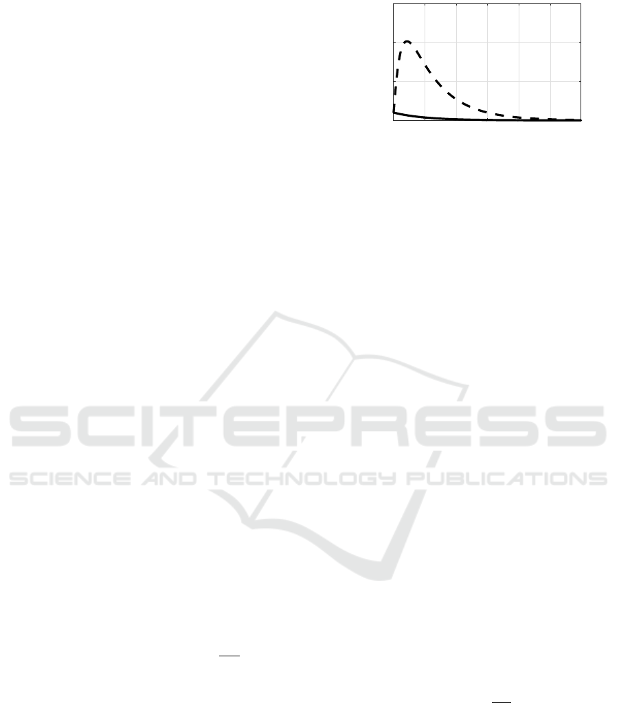
The norm behaviour of free motion of discrete-
time system (1) is depicted in Figure 1 for two cases
of the state matrix
¯
F.
0 50 100 150 200 250
k
0
5
10
15
||x(k)||
Figure 1: Norm of free motion of a stable discrete-time sys-
tem for different descriptions of the state matrix F
1
(dashed
line) and F
2
(solid line).
There are
¯
F
1
=

0.9802 1.3253
0 0.9139

and
¯
F
2
=

0.9471 0.0331
0.0331 0.9471

. It should be noted, the
eigenvalues
¯
λ
i
for both cases of
¯
F are the same:
¯
λ
1
= 0.9802,
¯
λ
2
= 0.9139. Obviously, norm be-
haviour with the matrix F
2
converges to zero mono-
tonically, while norm behaviour with the matrix F
1
has large deviation from the monotonic trajectory.
Here, the last case describes large deviation in the sys-
tem behaviour, that is the researched subject of the
paper.
Assessment of the upper bound of large deviations
of free motion of discrete-time system (1) is obtained
with representation of the state matrix
¯
F in the follow-
ing form
M
¯
Λ =
¯
FM, (4)
where
¯
Λ is a diagonal matrix of eigenvalues, M is a
square matrix whose columns are the n linearly inde-
pendent eigenvectors of
¯
F. Using (2) and (4), we get
M
¯
Λ
k
=
¯
F
k
M. (5)
Now, combining (2) and (5), we obtain
x(k) =
¯
F
k
x(0) = M
¯
Λ
k
M
−1
x(0). (6)
Let us form an upper bound of (3)
k
x(k)
k
=
w
w
w
M
¯
Λ
k
M
−1
x(0)
w
w
w
≤
k
M
k
w
w
w
¯
Λ
k
w
w
w
w
w
M
−1
w
w
k
x(0)
k
=
C
{
M
}
w
w
diag

¯
λ
k
i

;i = 1, n
w
w
k
x(0)
k
≤
C
{
M
}
¯
λ
k
max
k
x(0)
k
, (7)
where C
{
M
}
=
k
M
k
w
w
M
−1
w
w
is condition number
(Gantmacher, 1990), (Golub and Van Loan, 1996) of
the matrix M;
¯
λ
max
is a maximum eigenvalue of ma-
trix
¯
F that satisfies conditions Im

¯
λ
max

= 0,
¯
λ
max
>
0. Thus, by
k
x(0)
k
= 1 we have the upper bound:
sup(
k
x(k)
k
)
|
k
x(0)
k
=1
= C
{
M
}
¯
λ
k
max
. (8)
ICINCO 2020 - 17th International Conference on Informatics in Control, Automation and Robotics
644

It should be noted, if there is even one pair of close
to collinear eigenvectors, then the condition number
C
{
M
}
can be sufficiently large and, therefore, devia-
tion of free motion of the system become large also.
Main properties of equation (8) are discussed in
(Dudarenko et al., 2019).
3 DEVIATIONS IN
DISCRETE-TIME SYSTEMS
WITH CONTROL SIGNAL
DELAY
Any discrete-time control system is a composition
of following parts: digital controller, a digital-to-
analog converter, analog-to-digital converter and a
continuous-time plant. In order to obtain a single
mathematical description of this composition, pro-
cesses are studied at the time instances t = k · ∆t,
where k is positive integer, it is called the discrete
time; ∆t is the sample time. This means that the
discrete-time plant is said to be discrete time sampling
from continuous-time state and output variables under
a piecewise-constant control signal with the duration
∆t. Note that a control signal from the digital con-
troller can output both without delay and with delay
τ. This fact gives rise to two discrete-time representa-
tions of the continuous-time plant.
Consider a linear continuous-time plant:
˙
x(t) = Ax(t) + Bu(t); x(0),
y(t) = Cx(t), (9)
where x ∈ R
n
, u ∈ R
r
, y ∈ R
m
are state vector, in-
put vector, output vector respectively;A ∈ R
n×n
, B ∈
R
n×r
, C ∈ R
m×n
are state matrix, input matrix, output
matrix. If the control of the plant (9) for t = k · ∆t is
realized without delay, then it can be represented as
follows:
u(t) = u(k), k∆t ≤ t < (k + 1)∆t. (10)
Combining (9) and (10) (Zadeh and Desoer, 2008),
we get following discrete-time model of the plant:
x(k + 1) =
¯
Ax(k) +
¯
Bu(k); x(0),
y(k) =
¯
Cx(k), (11)
where k = arg(t = k∆t) is discrete time; ∆t
is sample time; dim

¯
A

= dim (A), dim

¯
B

=
dim(B), dim

¯
C

= dim(C),
¯
A = exp(A∆t),
¯
B =

¯
A − I

A
−1
B,
¯
C = C. Analytically, control (10) can
be written as:
u(k) =
¯
K
g
g(k) −
¯
Kx(k), (12)
where g ∈ R
m
is an external input;
¯
K
g
∈ R
r×m
,
¯
K ∈
R
r×n
are the feed forward matrix and the feedback
matrix respectively. Combining (12) and (9), we get
discrete-time closed-loop system:
x(k + 1) =
¯
Fx(k) +
¯
Gg(k); x(0),
y(k) =
¯
Cx(k),
ε(k) = g(k) − y(k), (13)
where
¯
F =
¯
A −
¯
B
¯
K,
¯
G =
¯
B
¯
K
g
, (14)
ε(k) is a tracking error. Eigenvalues and eigenvectors
of the state matrix is given by:
σ

¯
F

=

¯
λ
i
= exp(λ
i
∆t) : Im(
¯
λ
i
) = 0,
¯
λ
i
6=
¯
λ
j

,
(15)
¯
Fξ
i
=
¯
λ
i
ξ
i
;i = 1, n. (16)
The case of a discrete-time system with the control
signal delay is characterized by the increased dimen-
sion of the matrices and modification of eigenvector
structure of the state matrix. If the control u(t) of the
plant (9) for t = k ·∆t realizes with delay τ ≤ ∆t, then it
can be represented as follows (Grigoriev et al., 1983)
u(t) =

u(k − 1), k∆t ≤ t < k∆t + τ;
u(k), k∆t + τ ≤ t < (k + 1)∆t.
(17)
Combining (17) and (9), we get following discrete-
time model (Grigoriev et al., 1983) of the plant:
x(k + 1) =
¯
Ax(k) +
¯
B
1
(τ)u(k − 1) +
¯
B(τ)u(k);
y(k) =
¯
Cx(k), (18)
where
¯
B
1
(τ) =
¯
A

I − e
−Aτ

A
−1
B,
¯
B(τ) =

¯
Ae
−Aτ
− I

A
−1
B. (19)
Let us introduce an additional state vector χ, then we
get a following discrete-time model
˜
x(k + 1) =

x(k + 1)
χ(k + 1)

=

¯
A
¯
B
1
(τ)
0 0

x(k)
χ(k)

+

¯
B(τ)
I

u =
˜
A
˜
x(k) +
˜
Bu(k); y(k) =
˜
C
˜
x(k), (20)
where dim(χ) = dim(u) = r.
Two cases are considered. The first case is called
’unpredictable delay’ (or unaccounted delay). In this
case the control is the same like for discrete plant
without delay. That means an additional dimension
(Z
−1
is discrete-time operator) does not take into ac-
count when the control is designed. The control is
given by (12), but on account of the modification of
Robustness Estimation of Large Deviations in Linear Discrete-time Systems with Control Signal Delay
645

the plant model (20) the discrete-time system takes
the form:
˜
x(k + 1) =
˜
F
˜
x(k) +
˜
Gg(k); y(k) =
˜
C
˜
x(k), (21)
where
˜
F(τ) =

¯
A −
¯
B(τ)
¯
K
¯
B
1
(τ)
−
¯
K 0

,
˜
G(τ) =

¯
B(τ)
¯
K
g
¯
K
g

,
˜
C =

¯
C 0

(22)
Block diagram representation of system (21) with
control (12) is shown in figure 2.
Figure 2: Block diagram of system with unpredictable delay
in control.
The upper bound of free motion of system (21) takes
the form (8). And it should be noted that a change
of condition number C

˜
M

happens even by τ = 0
although eigenvalues set of the matrix
˜
F(τ) =
˜
F(0) is
increased a zero eigenvalue
˜
λ
n+1
= 0.
The second case is called ’predictable delay’ (or
accounted delay). In this case the control law takes
into account the additional dimension (Z
−1
discrete-
time operator) by an additional feedback
˜
K
χ
. The
control low for plant (20) takes the form
u(k) =
˜
K
g
g(k) −
˜
K
x
x(k) −
˜
K
χ
χ(k), (23)
Combining (20) and (23), we get the discrete-time
closed-loop system (21) with the next matrices
˜
F(τ) =

¯
A −
¯
B(τ)
˜
K
x
¯
B
1
(τ)−
¯
B(τ)
˜
K
χ
−
˜
K
x
−
˜
K
χ

,
˜
G(τ) =

¯
B(τ)
˜
K
g
˜
K
g

,
˜
C =

¯
C(τ) 0

(24)
Control law (23) is formed such that an eigenvalues
set of matrix
˜
F(τ) (24) consists of eigenvalues set of
matrix
¯
F (22) and an eigenvalue
˜
λ
n+1
. The eigen-
value
˜
λ
n+1
satisfies the condition
˜
λ
n+1

¯
λ
i
, i = 1, n.
Block diagram representation of system (21) with ma-
trices (24) and control (23) is shown in figure 3.
The upper bound of free motion of this system sat-
isfies the form (8) as well, where C

˜
M

is condition
number of (n + 1) × (n + 1) eigenvectors matrix
˜
M of
the state matrix
˜
F (24).
Figure 3: Block diagram of system with predictable delay
in control.
4 ROBUSTNESS ESTIMATION
Assume parameters of the state matrix linearly de-
pends on components of the vector of varying station-
ary parameters q = q
0
+ ∆q, q ∈ R
p
, where q
0
is vec-
tor of nominal value of the parameters q, ∆q is vector
of variations of the parameters. Then, the state matrix
¯
F(q) depends of the vector of varying parameters and
system (1) takes the following form:
x(k + 1, q) =
¯
F(q)x(k, q); x(0) = x(k, q)
|
k=0
, (25)
Therefore, equation (8) can be rewritten as:
kx(k, q)k≤ sup{kx(k, q)k}= C{M(q)}
¯
λ
k
max
(q)kx(0)k.
(26)
Consider a ν-sensitivity function Θ
ν
(k, q) of upper
bound (26) to variation of ν component of a vector
of parameters q
ν
. The sensitivity function Θ
ν
(k, q)
can be defined as:
Θ
ν
(k, q) =
∂(sup{kx(k,q)k})
∂q
ν



q
0
=

∂C{M(q)}
∂q
ν



q
0
¯
λ
k
max
+k
¯
λ
k−1
max
∂
¯
λ
max
(q)
∂q
ν



q
0
C{M(q)}

kx(0)k.
(27)
Note, calculation of derivative of conditional number
of the modified eigenvectors matrix C{M} = kMk ·
kM
−1
k depends on choosing norm. It is well known
(Gantmakher, 2010; Golub and Loan, 1996), the spec-
tral matrix norm is equal to maximum singular value
of the matrix, and the spectral norm of inversion of
the matrix is equal to inversion of minimum singular
value of the matrix
C{M} = kMk · kM
−1
k = α
M
{M} · α
−1
m
{M}, (28)
where α
M
{M}, α
m
{M} are maximum and minimum
singular values of matrix M respectively. If depen-
dency of the vector of parameters q for matrix M
is taken into account, equation (28) takes the form
C{M} = α
M
{M(q)} · α
m
{M(q)}. Then
∂C{M}
∂q
ν



q
0
=
∂α
M
{M}
∂q
ν



q
0
· α
−1
m
{M}−
α
M
{M}α
−2
m
{M}
∂α
m
{M}
∂q
ν



q
0
. (29)
ICINCO 2020 - 17th International Conference on Informatics in Control, Automation and Robotics
646

The parametric sensitivity function Θ
ν
(k, q) can be
calculated, if the sensitivity functions of singular val-
ues of the matrix of eigenvectors and the sensitiv-
ity functions of maximum eigenvalue of the state
matrix of system (25) are obtained. Full increment
∆sup{kx(k, q)k} of the upper bound (8) of the pro-
cess by the norm of the state vector of system (25) is
defined as
∆sup{kx(k, q)k} =
∑
p
ν=1
Θ
ν
(k, q
0
)∆q
ν
=
Θ
T
(k, q
0
)∆q, (30)
where Θ
T
(k, q
0
) = row{Θ
ν
(k, q
0
)};ν = 1, p. Obvi-
ously, the varying upper bound represents a composi-
tion of (8) and (30).
Based on the obtained equations, the following al-
gorithm for the robustness estimation of large devi-
ations in linear discrete-time system with parametric
uncertainties is proposed. The algorithm assumes that
parameters of the system are linearly dependent on
the uncertainties and has the following steps.
1. Define a discrete-time system with uncertainties
of parameters in form (25).
2. Calculate sensitivity matrix
∂
¯
F(q)
∂q
v



q
0
to variation
of parameter q
v
.
3. Calculate derivative of the maximum eigenvalues
of the state matrix of system according to
∂
¯
λ
max
∂q
v




q
0
= M
−1
∂
¯
F(q)
∂q
v




q
0
M
!
ii
(31)
4. Calculate sensitivity functions of maximum and
minimum singular values of the eigenvectors ma-
trix in relation to the next forms respectively
∂
∂q
v
α
M
{
M(q)
}|
q
0
= U
T
∂M(q)
∂q
v




q
0
V
!
11
,
(32)
∂
∂q
v
α
m
{
M(q)
}|
q
0
= U
T
∂M(q)
∂q
v




q
0
V
!
nn
,
(33)
where U and V are left and right singular basis of
singular value decomposition respectively
M = U

Σ = diag

α
i
; i = 1, n

V
T
. (34)
Matrix
∂M(q)
∂q
v
consists of sensitivity functions of
eigenvectors
∂M(q)
∂q
v




q
0
= row
(
∂M
i
(q)
∂q
v




q
0
;i = 1, n
)
, (35)
where
∂M
i
(q)
∂q
v




q
0
=
n
∑
k=1,k6=i
γ
v
ik
M
k
; γ
v
ii
= 0 (36)
and coefficients γ
v
ik
can be obtained as
γ
v
ik
=

M
−1
∂
¯
F(q)
∂q
v



q
0
M

ik
¯
λ
i
−
¯
λ
k
;k 6= i. (37)
5. Calculate the derivative of conditional number of
the eigenvectors matrix in form (29).
6. Form parametric sensitivity function of the upper
bound (27) of large deviation in discrete-time sys-
tem (25).
7. Find full increment of the upper bound of the pro-
cess according to (30).
8. Establish the curves of dependent of full incre-
ment of the upper bound of the process on discrete
time.
Note that a full increment ∆
¯
λ
max
(q) of maximum
eigenvalue can be calculated according to its sensi-
tivity function (31) such that
∆
¯
λ
max
=
p
∑
ν=1
∂
¯
λ
max
∂q
ν




q
0
∆q
ν
(38)
Then the full increment (30) taking into account sen-
sitivity function (27) and the full increment of the
maximum eigenvalue (38) can be defined as
∆sup{kx(k, q)k} =
p
∑
ν=1
Θ
ν
(k, q
0
, ∆
¯
λ
max
)∆q
ν
, (39)
where
Θ
ν
(k, q
0
, ∆
¯
λ
max
)


kx(0)k=1
=
∂C{M(q)}
∂q
ν



q
0
(
¯
λ
max
+ ∆
¯
λ
max
)
k
+
C{M(q)}k(
¯
λ
max
+ ∆
¯
λ
max
)
k−1
∂
¯
λ
max
(q)
∂q
ν



q
0
. (40)
Finally an upper bound sup{kx(k, q)k} of the process
kx(k, q)k is estimated by (8) and (40) as follows
sup{kx(k, q)k}
|
kx(0)k=1
=
C{M}(
¯
λ
max
+ ∆
¯
λ
max
)
k
+
∆sup{kx(k, q)k}. (41)
5 ROBUSTNESS ESTIMATION OF
DEVIATION UNDER
UNCERTAINTY OF DELAY IN
CONTROL
Suppose that q is variation of delay
q = τ = τ
0
+ ∆τ, (42)
Robustness Estimation of Large Deviations in Linear Discrete-time Systems with Control Signal Delay
647

where τ
0
= 0; ∆τ = (0; ∆t]. Then variations of large
deviations can be estimated according to the proposed
algorithm. Using the algorithm we can estimate upper
bound variation (8) depending from changes of con-
trol signal delay. The main point is to get sensitivity
matrix of the state matrix of the discrete-time closed-
loop system from section 3.
Consider the above two cases. For unpredictable
delay we get following sensitivity matrix of state ma-
trix (22)
∂
˜
F(τ)
∂τ



τ
0
=

−
∂
¯
B(τ)
∂τ
¯
K
∂
¯
B
1
(τ)
∂τ
0 0





τ
0
=

¯
AB
¯
K
¯
AB
0 0

. (43)
For predictable delay the sensitivity matrix of state
matrix (24) takes the form
∂
˜
F(τ)
∂τ



τ
0
=

−
∂
¯
B(τ)
∂τ
˜
K
x
∂
¯
B
1
(τ)
∂τ
−
∂
¯
B(τ)
∂τ
˜
K
χ
0 0





τ
0
=

¯
AB
˜
K
x
¯
AB(1 +
˜
K
χ
)
0 0

. (44)
According to the algorithm, these matrices are the ba-
sis for next ensuing calculations of sensitivity func-
tions of eigenvalues (31), eigenvectors (36), singular
values (32), (33) and as result the upper bound (41).
6 EXAMPLE
Consider a stable continuous plant (9) with matrices
A =

0 1
−0.01 −0.2

;B =

0
1

;C =

1 0

.
Let us design a discrete-time system for the plant
with sample time ∆t = 0.01s using modal control with
desired eigenvalues σ(
¯
F) = {0.9802, 0.9139}. The
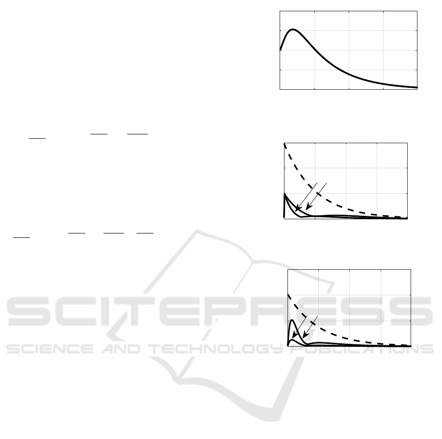
discrete-time system without control signal delay is
described. There is a deviation of free motion of the
system, that is shown on the Fig.4, where deviation
achieves max kx(k)k=1.536. Note, in this example the
norm of the vector of initial conditions equals one
kx(0)k = 1 for all cases. Then let us consider the
above two cases of presence of delay in control sig-
nal.
6.1 The Case of Unpredictable Delay of
Control Signal
For the case of unpredictable control signal delay the
system (21) is described with matrices (22). The Fig.5
0 50 100 150
k
0
0.5
1
1.5
2
||x(k)||
Figure 4: Norm of free motion of the discrete-time system
without control signal delay.
0 50 100 150
k
0
20
40
60
||x(k)||
1
2
Figure 5: Norm of free motion and upper bound estimation
of the discrete-time system with unpredictable delay.
0 50 100 150
k
0
50
100
150
||x(k)||
1
2
Figure 6: Norm of free motion and upper bound estimation
of the discrete-time system with predictable delay.
shows norms of free motion for delays τ = 0.1∆t
(curve 1),τ = 0.3∆t (curve 2) and the upper bound
(41) for τ = 0.3∆t.
The deviation achieves max kx(k)k = 20. It should
be noted the system becomes unstable for τ > 0.45∆t.
6.2 The Case of Predictable Delay of
Control Signal
For the case of predictable control signal delay the
system (21) is described with matrices (24) and ad-
ditional desired eigenvalue for control law (23) is
¯
λ
3
= 0.8187. The Fig.6 shows norm of free motion
for delays τ = 0.1∆t (curve 1),τ = 0.3∆t (curve 2) and
the upper bound (41) for τ = 0.3∆t.
The deviation achieves max kx(k)k = 51.8 and the
system stays stable. Obviously, the value of the delay
in both cases affects the level of deviation in free mo-
tion of the discrete-time system. Moreover, the pre-
dictable control signal delay has biggest influence on
ICINCO 2020 - 17th International Conference on Informatics in Control, Automation and Robotics
648

the level of deviation than unpredictable control sig-
nal delay, but stability is guaranteed.
7 CONCLUSIONS
The aim of the paper was to get estimation of ro-
bustness of large deviations in free motion of stable
linear discrete-time systems with parametric uncer-
tainties. The tracking discrete-time system with pre-
dictable control signal delay and unpredictable con-
trol signal delay was considered in the paper. Using
a combination of state-space approach and the sensi-
tivity theory methods the estimation robustness of the
large deviations was obtained. It was derived that the
upper bound by the norm of the large deviations in lin-
ear discrete-time systems with parametric uncertain-
ties depends of sensitivity functions of singular values
of the eigenvectors matrix of the system state matrix.
At the same time the sensitivity matrix of a state ma-
trix depends on the value of the control signal delay,
and that relationship was obtained. The algorithm for
robustness estimation of the large deviations was pro-
posed and the illustrative example was given. It was
shown, that the predictable control signal delay has
biggest influence on the level of deviation than unpre-
dictable control signal delay, but stability is guaran-
teed.
In future, it is supposed to expand the results of
the paper to the case of a discrete-time systems with
parametric uncertainties having complex eigenvalues.
ACKNOWLEDGEMENTS
This work was financially supported by Government
of Russian Federation, Grant 08-08.
REFERENCES
Abidi, K. and Soo, H. (2019). Discrete-time adaptive regu-
lation of systems with uncertain upper-bounded input
delay: A state substitution approach. In Proceedings
of the 16th International Conference on Informatics in
Control, Automation and Robotics, pages 699–706.
Ahiyevich, U., Parsegov, S., and Shcherbakov, P. (2018).
Upper bounds on peaks in discrete-time linear sys-
tems. volume 79, pages 1976–1988.
Dudarenko, N., Vunder, N., and Grigoriev, V. (2019). Large
deviations in discrete-time systems with control signal
delay. In in Proceedings of 16th International Con-
ference on Informatics in Control, Automation and
Robotics, pages 281–288.
Eslami, M. (1994). Theory of Sensitivity in Dynamic Sys-
tems: An Introduction. Springer-Verlag, Berlin.
Feldbaum, A. (1948). On the distribution of roots of char-
acteristic equations of control systems. In Avtomatika
i Telemekhanika, volume 4, pages 253–279.
Gantmakher, F. (2010). Matrix Theory. Fizmatlit Publ.,
Moscow.
Golub, G. and Loan, C. V. (1996). Matrix Computations.
Johns Hopkins University Press, Baltimore.
Grigoriev, V., Drozdov, V., Lavrentiev, V., and Ushakov, A.
(1983). Synthesis of discrete regulators by computer.
Mashinostroenie, Leningrad.
Izmailov, R. (1987). The peak effect in stationary linear
systems with scalar inputs and outputs. In Automation
and Remote Control, volume 48, pages 1018–1024.
Khlebnikov, M. (2018). Upper estimates of the deviations
in linear dynamical systems subjected to uncertainty.
In in 15th International Conference on Control, Au-
tomation, Robotics and Vision, ICARCV 2018, pages
1811–1816.
Liberzon, D. (2003). Switching in systems and control.
Birkhauser, Boston.
Liu, B., Huang, J., Yang, M., and Liu, D. (2018). Expo-
nential stabilization via event-triggered control for lin-
ear discrete-time delayed systems. In Proceedings of
the 2018 Chinese Control And Decision Conference
(CCDC), pages 4700–4704.
Margun, A. and Furtat, I. (2016). Robust control of uncer-
tain linear plants in conditions of signal quantization
and time-delay. In Proceedings of the 13th Interna-
tional Conference on Informatics in Control, Automa-
tion and Robotics, pages 514–520.
Polotskij, V. (1981). Estimation of the state of single-output
linear systems by means of observers. In Automation
and Remote Control, volume 41, pages 1640–1648.
Polyak, B. and Smirnov, G. (2016). Large deviations for
non-zero initial conditions in linear systems. In Auto-
matica, volume 74, pages 297–307.
Polyak, B., Tremba, A., Khlebnikov, M., Shcherbakov, P.,
and Smirnov, G. (2015). Large deviations in linear
control systems with nonzero initial conditions. In Au-
tomation and Remote Control, volume 76, pages 957–
976.
Shcherbakov, P. (2017). On peak effects in discrete time lin-
ear systems, in 5th mediterranean conference on con-
trol and automation. In in 5th Mediterranean Confer-
ence on Control and Automation, MED 2017, pages
376–381.
Sussman, H. and Kokotovic, P. (1991). The peaking phe-
nomenon and the global stabilization of nonlinear sys-
tems. In IEEE Trans. Automat. Control, volume 36,
pages 461–476.
Tou, J. (1964). Modern Control Theory. Mc. Graw-Hill
Book Company, INC, New York.
Vunder, N. and Dudarenko, N. (2018a). Analysis of system
situations with a non-zero initial state in the task of
pre-operational adjustment of the main reflector of a
large full-rotary radio telescope. In Journal of Optical
Technology, volume 10, pages 33–42.
Robustness Estimation of Large Deviations in Linear Discrete-time Systems with Control Signal Delay
649

Vunder, N. and Dudarenko, N. (2018b). Robustness es-
timation of free motion deviations of aperiodic sys-
tems with sensitivity theory methods. In Scientific and
Technical Journal of Information Technologies, Me-
chanics and Optics, volume 18, pages 704–707.
Vunder, N., Nuyya, O., Pescherov, R., and Ushakov, A.
(2016). Research of free motion trajectories features
of continuous system defined as a consecutive chain of
identical first-order aperiodic links. In Scientific and
Technical Journal of Information Technologies, Me-
chanics and Optics, volume 16, pages 68–75.
Vunder, N. and Ushakov, A. (2015). On the features of the
trajectories of autonomous discrete systems generated
by a multiplicity factor of eigenvalues of state matri-
ces. In in Proceedings of IEEE International Sympo-
sium on Intelligent Control, pages 695–700.
Vunder, N. and Ushakov, A. (2017). The problem of form-
ing the structure of eigenvectors of state matrix of con-
tinuous stable system which guarantees the absence
of deviation of its trajectories from monotonically de-
creasing curve of free motion. In Journal of Automa-
tion and Information Sciences, volume 49, pages 27–
40.
Zadeh, L. and Desoer, C. (2008). Linear system theory: the
state space approach. New York: Dover Publications,
New York.
ICINCO 2020 - 17th International Conference on Informatics in Control, Automation and Robotics
650