
Optimal Path Planning for Drone Inspections of Linear Infrastructures
Golizheh Mehrooz and Peter Schneider-Kamp
Dept. of Mathematics & Computer Science, University of Southern Denmark, Denmark
Keywords:
Path Planning, Routing, A* Algorithm, Drone Inspections, Power Grids.
Abstract:
Autonomous Beyond Visual Line of Sight (BVLOS) flights represent a huge opportunity in the drone industry
due to their ability to monitor larger areas. Autonomous navigation and path planning are essential capabil-
ities for BVLOS flights. In this paper, we introduce the routing component of a path planning system for
inspecting linear infrastructures. We explore both a direct algorithm and a transformation algorithm. The
direct algorithm is an extension of A* to allow limited routing through air as well as the use of non-logic
intersections. The transformation algorithm pre-computes a graph that include edges for routing through air
and nodes for non-logic intersections. We implemented both algorithms for routing along a particular type of
linear infrastructure, power lines, and validated them through an empirical evaluation at three different scales:
the Danish power grid, the French power grid, and the entire European power grid. The test results show that
the transformation algorithm allows for sub-second routing performance for a small-to-medium sized power
grid. Larger power grids can be routed in less than five seconds, and even an optimal route of more than six
thousand kilometers along linear infrastructures from Portugal to Sweden via Russia is found in less than half
a minute. All algorithms have been implemented and are available as an open-source Python package for
Linear-infrastructure Mission Control (LiMiC).
1 INTRODUCTION
There are more than 200,000 km (University of
Southern Denmark, ) of overhead power line cables
in European countries that are the backbone of the en-
ergy infrastructure. According to ((Mrs.), ), a heavy
windstorm, which caused a tree to fall on an important
power line in Switzerland, resulted in around $1.2 bil-
lion worth of damage. Approximately 56 million peo-
ple – mainly in Italy but also in Switzerland – were
without power for several hours ((Mrs.), ). Thus, in
order to prevent power outages, electric utilities regu-
larly perform inspections of their power grids to plan
for the necessary repair or replacement work (Nguyen
et al., 2019).
To improve the inspection speed, accuracy, safety,
and costs, a considerable amount of research has been
conducted in order to automate inspections by us-
ing drones. Drones have been used in various ar-
eas such as infrastructure inspections for automating
labor-intensive, time-consuming, and sometimes even
dangerous tasks. However, the current applications
of drones in the area of inspecting linear infrastruc-
tures such as power lines still face many unsolved
challenges such as drone flight time as well as au-
tonomous BVLOS flights.
The BVLOS flights represent a huge opportunity
in the drone industry especially in the field of linear
infrastructure inspection due to their ability to mon-
itor larger areas. During a BVLOS flight, the drone
often flies out of the visual range of the Pilot-in-
Command. Thus, extra safety features such as the
capability to autonomously navigate and path plan-
ning have to be considered on the drone to prevent
the aircraft from flying beyond the restricted area as-
signed by the Special Flight Operations Certificates
(SFOC)(Fang et al., 2018).
The core task of autonomous navigation and path
planning for linear infrastructures is optimal routing,
i.e. finding the shortest path along the infrastruc-
ture between two given elements of the infrastructure.
This task is very important not only for routing drones
from one location to another, but, more importantly,
also as the basic building block of other tasks such as
optimal scheduling of inspection missions. For practi-
cal purposes of mission control for drone inspections,
we aim as a design goal for the routing algorithm to
run in less than one second.
New EU regulations for drone inspections have
ease the process of obtaining permission to fly inspec-
tion missions for the special case of inspecting linear
326
Mehrooz, G. and Schneider-Kamp, P.
Optimal Path Planning for Drone Inspections of Linear Infrastructures.
DOI: 10.5220/0009846703260336
In Proceedings of the 6th International Conference on Geographical Information Systems Theory, Applications and Management (GISTAM 2020), pages 326-336
ISBN: 978-989-758-425-1
Copyright
c
2020 by SCITEPRESS – Science and Technology Publications, Lda. All rights reserved
infrastructures. These regulations require the drone
to stay within close range to the linear infrastructure
(world, ). Thus, finding an optimal route requires con-
sidering many factors such as minimizing the flight
time a drone spends away from the immediate vicin-
ity of the linear infrastructure. This factor can be rep-
resented through a cost function that penalizes flying
away from the linear infrastructure and, thus, affects
which route is considered optimal.
There are standard solutions for routing in road
networks. The Open Source Routing Machine
(OSRM) (Huber Stephan, 0601) is an open-source
C++ implementation of a high-performance routing
engine for finding the shortest path in such a network,
and it is available as a light-weight docker image for
straightforward deployment.
In the case of power line inspections considered
in this paper, we can view the optimal routing prob-
lem along linear infrastructures as a search problem
for finding a path with a minimum cost between
two power towers, including possibly limited rout-
ing through air and the use of non-logical intersec-
tions. This search problem poses several significant
challenges, which effectively preclude the use of pre-
existing routing solutions such as OSRM:
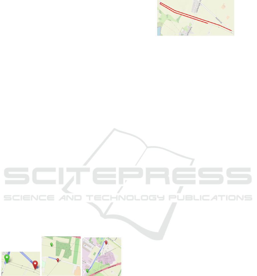
• The start and end power towers are on different
parallel power lines. (see Fig. 1 (a)).
• There is an intersection between power lines, and
the start and end power towers are on these lines.
(see Fig. 1 (b)).
• The lines intersect with no-fly zones (e.g. around
airports) or infrastructure to be avoided (e.g.
transformer stations, power plants). (see Fig. 1
(c)).
(a) Parallel points (b) Intersection (c) Power substation
Figure 1: Path planning challenges.
In Fig. 1 (a), the start and end power towers are on
two parallel power lines. In order to find a path be-
tween these two power towers, one might be tempted
to use OSRM with a profile for drones that use power
lines instead of streets. The result of such a routing is
shown in Fig. 2.
The route computed by OSRM starts from the star
power tower and follows the line until it arrives at a
transformer substation. From the substation, it routes
Figure 2: Path planning by using OSRM.
within the transformer substation to the other power
line and follows that one until it reaches the end power
tower. It is immediately apparent that OSRM can-
not find the shortest path between these two power
towers, and that it only finds a path due to the two
power lines being logically connected through the
transformer station.
In the case of Fig. 1 (b), OSRM cannot find a route
as the two power lines are logically never connected.
In both Fig. 1 (a) and (c), a route computed by OSRM
would require the drone to fly through a transformer
station. This is undesirable for a multitude of safety
reasons. Due to these problems, we could not use
OSRM or similar pre-existing solutions for optimal
routing.
In order to solve these problems, we have imple-
mented two algorithms to compute the shortest path
between two elements of a linear infrastructure such
as power lines: (1) a direct algorithm based on an ex-
tension of the A* algorithm for finding the shortest
paths in weighted graphs as well as (2) a transforma-
tion algorithm for transforming the special conditions
of the problem into a standard weighted undirected
labelled graph.
The direct algorithm extends the A* algorithm
by allowing to route between two nodes not con-
nected through an explicit edge with certain restric-
tions: routing through air is penalized by having a
higher cost factor and is allowed only up to a certain
distance to take into account regulatory restrictions.
Furthermore, given that the edges of our graph are on
an essentially two-dimensional surface, they might in-
tersect. Thus, the algorithm also has to find intersec-
tions and use them to change from one power line to
another without having to fly away from the power
lines.
The transformation algorithm builds on the same
ideas as the direct algorithm but pre-computes a graph
of power towers. The nodes of the graph are locations
typically representing power towers. The edges of the
graph are weighted by the distance between two con-
nected power towers. There are also edges connect-
ing power towers through air with scaled weights to
model higher costs. Finally, there are nodes repre-
senting non-logical intersections of power lines. An
optimal route between two power towers then corre-
sponds to the shortest path between two nodes in the
Optimal Path Planning for Drone Inspections of Linear Infrastructures
327

graph, and it can be found by using standard graph
algorithms such as the A* algorithm.
The rest of this paper is structured as follows: Sec-
tion 2 presents and explores the direct algorithm, in-
cluding how to speed up repeated calculations and
queries to the map data through various caching
schemes and the use of multi-threading. Section 3
presents and explores the transformation algorithm
for optimal routing which allows the use of standard
shortest path algorithms, including different pruning
methods for removing redundant edges in the graph.
Sections 4, 5, and 6 illustrate the results of the em-
pirical evaluations on the Danish, the French, and the
European power grids. Section 7 concludes this paper
and discusses possible future work.
2 THE DIRECT ALGORITHM
This section presents and explores the direct algo-
rithm, including how to speed up repeated calcula-
tions and queries to the map data through various
caching schemes and the use of multi-threading.
2.1 The Extension of A* to Route
through Penalized Air and to
Consider Non-logical Intersections
The A* (pronounced “a star”) algorithm(Ducho
ˇ
n
et al., 2014) is a popular choice for path planning
problems, as it is guaranteed to return an optimal so-
lution and can be used in a wide range of contexts.
It combines the speed of heuristic approaches like
Greedy Best-First-Search (Dechter and Pearl, 1985)
and optimal approaches such as Dijkstra’s algorithm
(Noto and Sato, 2000). The A* algorithm begins with
the start node and successively computes the exact
cost of the path from the starting node to any other
node n represented as a function g(n). In order to se-
lect which n to expand next, A* employs a heuristic
based on the estimated cost from node n to the end
node represented as h(n). When the end point n
end
is reached, the A* algorithm terminates. The cost
is then known through g(n
end
), and the path repre-
senting the corresponding route can easily be recon-
structed through a simple bookkeeping exercise. As
long as the heuristic function h is admissible (i.e., it
underestimates the costs to the end node), the cost and
route found by A* are guaranteed to be optimal.
In (Sathyaraj, 2008), authors compare the A* al-
gorithm with Dijkstra solver and Floyd-Warshall al-
gorithm in the term of the increasing number of nodes
visited and the time of computation consumed. As, in
the worst-case, the Dijkstra algorithm has to consider
all paths to all possible nodes, the time complexity of
that algorithm depends on the number of nodes and
edges in the graph. However, the time complexity of
the A* algorithm does not depend on the total num-
ber of nodes(Sathyaraj, 2008) but only on the length
of the shortest path and the average branching factor.
The Floyd-Warshall algorithm computes the shortest
paths between all nodes. On large sparse graphs such
as the ones representing linear infrastructures, this is
prohibitive in terms of time and space requirements.
In (Sathyaraj, 2008), authors concludes that the A* is
the best-established general algorithm for finding op-
timal routes.
The variant of the A* algorithm proposed in this
paper has several parameters:
• SafeDist: the minimum distance to keep from
perilous infrastructure such as transformer sta-
tions
• MaxFly: the maximum free flying distance away
from infrastructure elements such as power towers
• Penalty: the penalty factor for flying away from
infrastructure elements
• Precision: when set to larger than 1, the algorithm
will perform faster but find possibly non-optimal
routes
The SafeDist parameter has two functions: it makes
the drone avoid infrastructure elements such as trans-
former stations, and it avoids unnecessary routing
complexity, as transformer stations internally consist
of a large number of logical and non-logical intersec-
tions and, consequently, increase the average branch-
ing factor. We use a default value of 100 metres.
For the MaxFly parameter, we set a default of
1000 metres, which again has two effects: it disal-
lows flying away from power towers for more than
1 km, and it keeps the average branching factor on
a somewhat manageable level. In our initial experi-
ments, we found that a much lower value would suf-
ficie for most situations. But there are situations such
as flying around a transformer station or crossing over
to a line, where free flights of up to a few hundred
metres were necessary to avoid having to add tens or
hundreds of kilometres.
The Penalty parameter is used to penalize such
free flying time away from power lines. We use a
default value of 20, as we would rather have the drone
fly for an extra kilometre than have it fly 100 metres
away from the power lines.
The Precision parameter scales the estimate for
h(n). We use a default value of 1, as we strive for
fully optimal routes in order to keep flying times for
the drones minimal.
GISTAM 2020 - 6th International Conference on Geographical Information Systems Theory, Applications and Management
328
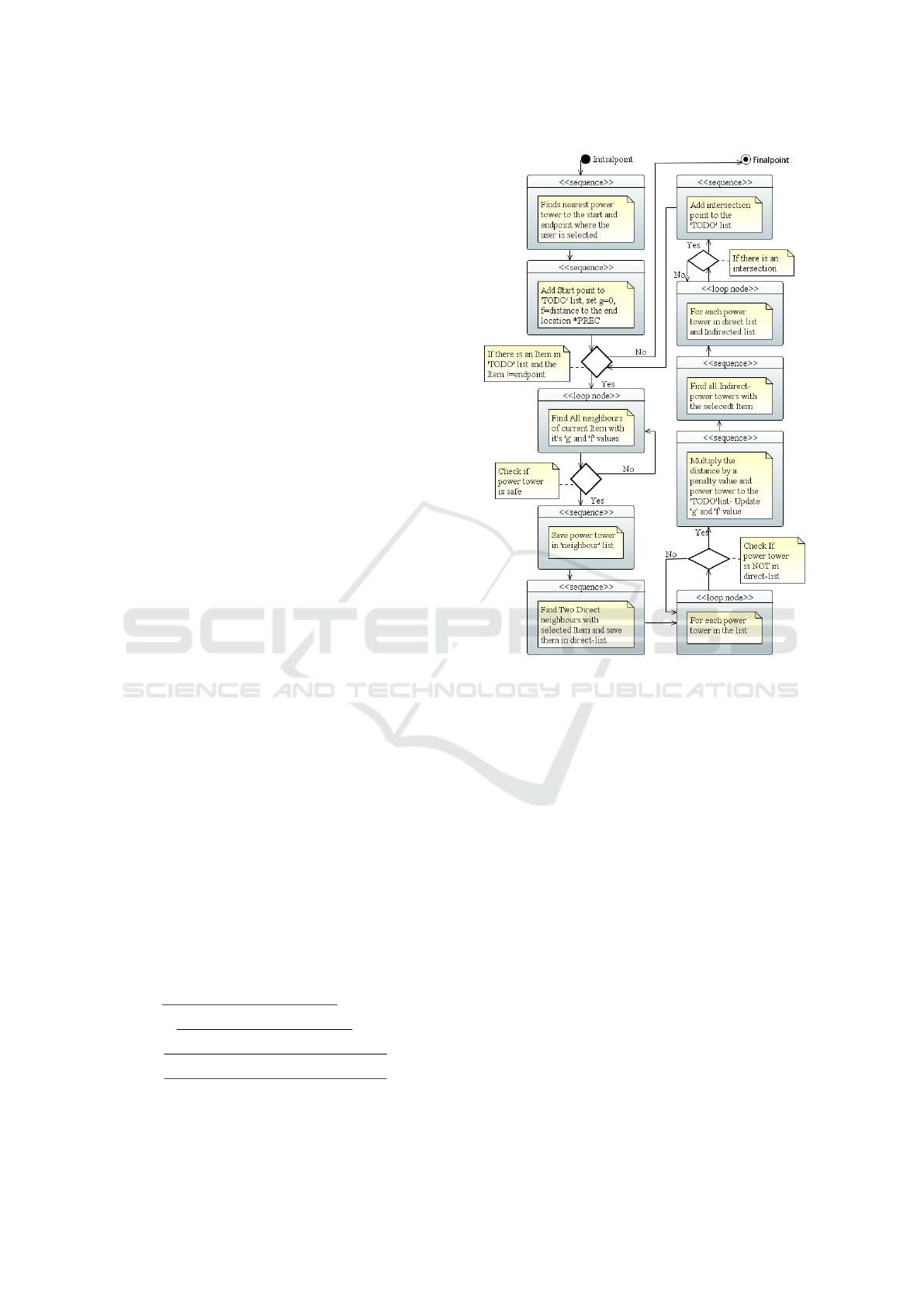
Fig. 3, shows the UML diagram of the direct A*
algorithm. As shown here, the algorithm finds the
nearest power towers to the start and end points se-
lected by the user. In this algorithm, we have a pri-
ority queue of power towers to visit called the TODO
list. The power towers in the queue are sorted by their
f -value, i.e., by their estimated total costs. The algo-
rithm is executed until the queue is empty or the least
costly element of the queue is equal to the endpoint.
In the beginning, we add the start power tower to the
TODO queue with the g-value set to zero and the f -
value set to the distance between the start and the end
tower multiplied by the Precision value. For example,
in the beginning, the queue contains the following in-
formation:
(dist=320.89,tower=pylon(id=831295194,
latlon=(55.3466014,
10.447012),neighbours=())). Here, dist is the
f -value and pylon is the class we use to hold
the id, GPS location, and possibly neighbours of
intersections.
Then for the most promosing item in the TODO
queue, the algorithm finds all the direct neighbors of
the tower as well as all other towers within MaxFly
distance. Only the neighbours which are safe accord-
ing to SafeDist are kept. The g-value and h-values
are computed, the g-values are scaled by the Penalty
factor.
The algorithms divides the neighbours into power
towers on the same line (direct neighbours) and those
that are not (indirect neighbours). Then it calculates
possible intersections between the power line seg-
ments between the current tower and its direct neigh-
bours and the segments between indirect neighbours.
Given that these towers are in close proximity, we
compute possible intersections using a standard for-
mula for intersections in a plane. The formula com-
putes the intersection of the infinitely long lines con-
taining the segments represented by the coordinates
of the four power towers - (x
1
,y
1
) and (x
2
,y
2
) for the
direct segment and (x
3
,y
3
) and (x
4
,y
4
) for the indi-
rect segment. Here, d is the denominator used and 0,
if the segments/lines are parallel. Otherwise, t and u
compute whether the intersection is on the segments
(0 ≤ t,u ≤ 1). If the intersection is on the segments,
the intersection coordinates x and y can be computed.
d = (x
1
− x
2
) ∗ (y
3
− y
4
) − (y
1
− y
2
) ∗ (x
3
− x
4
)
t =
(x
1
−x
3
)∗(y
3
−y
4
)−(y
1
−y
3
)∗(x
3
−x
4
)
d
u = −
(x
1
−x
2
)∗(y
1
−y
3
)−(y
1
−y
2
)∗(x
1
−x
3
)
d
x =
(x
1
∗y
2
−y
1
x
2
)∗(x
3
−x
4
)−(x
1
−x
2
)∗(x
3
y
4
−y
3
x
4
)
d
y =
(x
1
∗y
2
−y
1
x
2
)∗(y
3
−y
4
)−(y
1
−y
2
)∗(x
3
y
4
−y
3
x
4
)
d
The above approach for computing the shortest
path is very slow in practice due to the large number
Figure 3: UML Activity diagram of the direct algorithm.
of web-service requests to the overpass API. In the
next subsections, we explain about how to use a disk-
based cache file and a memory based-cache file in or-
der to cache web-service requests in order to speed up
the shortest path calculations.
2.2 Speeding Up Repeated Calls and
Calculations through a Disk-based
Cache
In order to speed up the performance of the algo-
rithm, our first attempt was to employ a disk-based
cache for storing information persistently. In this
case, we have used the dogpile.cache module. A
dogpile lock allows a single thread to generate an
expensive resource while other threads use the “old”
value until the “new” value is ready(python library,
). The dogpile.cache module provides an interface
to caching backends of any variety. The DBM file
backend uses a lock-file alongside a Unix-style DBM
file. A lock file is used to protect the DBM file itself
from concurrent writes and for coordinating the value
creation. A cache in the dogpile.cache framework
Optimal Path Planning for Drone Inspections of Linear Infrastructures
329

consists of a region, a backend, and value generating
functions. A region is an instance of the cache region
class and defines the configuration details for a partic-
ular cache backend. A backend describing how val-
ues are stored and retrieved from a backend. Finally,
data generation functions are user-defined functions
that generate new values to be placed in the cache.
In this research, the data generation func-
tions generate new values by requesting
data through overpass API. we have used
@region.cache on arguments() as a decora-
tor function for these functions for fully-transparent
querying and updating of the cache. For instance, the
find neighbours id function sends the following
query for finding the locations of all power towers
on the same power line as power tower with id
1881623946:
https://overpass.kumi.systems/api/interpreter?data=
[out:json][timeout:3600];(node(id:1881623946)
;way(bn)[”power”=”line”];node(w););out;
The code below exemplifies how we use
dogpile.cache in this paper. We have de-
fined a region which uses a file astar.dbm as a
backend for storing and retrieving data. ”@re-
gion.cache
on arguments()” on the top of the
”find towers” function is used for updating the
“astar.dbm” cache file.
region = dogpile.cache.make_region()
.configure("dogpile.cache.dbm",
arguments={"filename":"astar.dbm"})
@region.cache_on_arguments()
def find_neighbours_id(location, around):
return (towers);
In the next subsection, we explain how to use a
memory-based cache with a persistence layer as well
as how multi-threading can be used to pre-fill the
cache file.
2.3 The Pre-filling of a Persistent
Memory-based Cache
As we mentioned in the previous section, in order
to increase the speed of path planning, we have em-
ployed a disk-based cache. In this section we explain
how to use a memory-based cache instead. We have
decided to use a memory-based cache, as the loading
of cache data from a disk and the locking mechanism
are both rather slow compared to loading the cache
data from the memory.
Python’s standard perstistence layer Pickle can
be used to serialize and deserialize a Python object
structure. In this research, we have used Pickle
for loading the dictionaries that serve as backend for
memory-based caches in dopgile.cache. Unpickle
is used to open the cache file for reading. The fol-
lowing code shows how the cache data is saved and
loaded.
# saving cache file to astar.cache
pickle.dump(region.backend._cache,
open("astar.cache","wb"))
# load cache file to the region
region.backend._cache = pickle.load(
open("astar.cache","rb"))
Table 1 shows times for picking and unpickling
different file types in seconds. Not compressing
(None) is the fastest choice for both saving and load-
ing file. Compressing with gzip is a good compro-
mise, when the focus is on fast loading and reasonable
file size. Pickling and unpickling times for xz, which
produces the smallest file size, are highest compared
to other options.
Table 1: Time for pickling and unpickling different files.
Compression Size Pickling (seconds) Unpickling (seconds)
None 368,318K 12.845 28.538
gzip 153,148K 84.380 35.121
bz2 145,436K 45.494 43.844
xz 102,099K 159.424 46.912
In the next subsection, we explain about using
multi-threaded for pre-filling the cache.
2.4 The Multi-threaded Pre-filling of
the Cache
A thread of execution is defined in computer science
as the smallest sequence of programmed instructions
that can be scheduled in an operating system. Multi-
threaded programs run faster on computer systems
because these threads can be executed concurrently.
Threads of the process share the memory of the global
variables. If the global variables change in one thread,
this change is valid for all threads.
The concurrent.futures module in Python 3
provides a high-level interface for asynchronously
executing “callables”, typically functions with pa-
rameters. The asynchronous execution can be per-
formed with threads using the ThreadPoolExecutor
class. An Executor object uses a pool of at
most max workers threads to execute calls asyn-
chronously.
In this research, we used multiple threads for pre-
filling our cache, allowing to submit multiple Over-
pass queries simultaneously to the server. The code
bellow illustrates this multi-threaded approach for
pre-filling the cache.
import concurrent.futures as cf
exe = cf.ThreadPoolExecutor(max_workers)
exe.submit(find_all_neighbours, tower,
around, safe_dist))
GISTAM 2020 - 6th International Conference on Geographical Information Systems Theory, Applications and Management
330
In the next section, we explain the implementation
of the transformation algorithm for routing.
3 THE TRANSFORMATION
ALGORITHM
This section is split threefold. In the first subsec-
tion, we explain about extracting the graph from
the memory-based cache file which we have cre-
ated by multi-threaded pre-filling in the previous sec-
tion. In the second subsection, we use two functions
(prune complete and prune incomplete) for prun-
ing the redundant edges in the graph. In the third sub-
section, we use standard A* implementations on the
graph for routing.
3.1 Extracting a Weighted Undirected
Graph Including Non-logical
Intersections and Penalized Air
A weighted labelled graph G is a set of nodes N la-
belled by a function ` connected by edges E weighted
by a function w(e). It can be represented as G =
(N, E,`,w). The nodes N in this research are la-
belled with power tower GPS locations from the
map. Two nodes n
1
,n
2
∈ N are connected by an
edge e
d
= (n
1
,n
2
) ∈ E if there is a power line be-
tween these two locations. This edge is labelled
with a weight that represents the distance between
the two locations, i.e., w(e
d
) = distance(`(n
1
),`(n
2
))
where we use the Haversine distance function for
distance. There is also an edge e
i
between two nodes
n
1
,n
2
∈ N if distance(n
1
,n
2
) < around. In this case,
such an edge e
i
= (n
1
,n
2
) ∈ E would be labelled
with the penalized distance, i.e., w(e
i
) = penalty ×
distance(`(n
1
),`(n
2
)).
A path through a graph is a traversal of the con-
secutive nodes along a sequence of edges (Sathyaraj,
2008). The length of the path is the sum of the weights
of edges that are traversed along the path. The best
path is the one which has the minimum sum of the
weights from the source to the destination.
Path planing is the determination of all possible
paths from the start point to the endpoint and it is the
art of deciding which path to take. This decision is
based on the length of the path. Therefore, path plan-
ing depends on factors including how to get from the
starting point to the end, how to get around obstacles
in the way and how to find the shortest possible path.
(Sathyaraj, 2008).
Different methods have been developed to solve
this problem and find the shortest path such as the
unidirectional A*, the bidirectional A*, the Floyd-
Warshall (Hougardy, 2010), and the Dijkstra’s algo-
rithm. Standard graph packages such as networkx
support all these algorithms. We use networkx
for generating the shortest path in the graph of
power towers as we found it to have better out-of-
the-box performance than competitors such as e.g.
graph tool (graph tool, ).
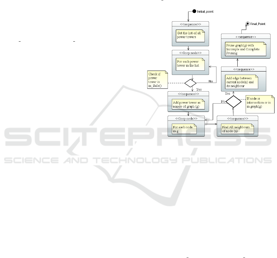
Figure 4: UML Activity diagram of extracting graph.
Fig. 4 shows the UML diagram for extracting the
graph. In this research, we have created a graph of
power towers for each European country. First, we
send an overpass API request to get the list of all
power towers for the specific European country. Then
for each power tower in the list, the algorithm checks
if the power tower is in a safe distance from power
substations. If this is the case, it adds the power tower
as a node of the graph. For adding the edges between
nodes the algorithm finds all direct and indirect neigh-
bors of the current power tower with their distance.
The algorithm is also creating non-logical intersec-
tion points in the graph and adds edges between these
points and the current power tower. We also use two
functions prune
complete and prune incomplete
to remove edges that can never be part of a shortest
path. This increases the performance of the transfor-
mation algorithm. We explain these functions in the
next subsection.
Optimal Path Planning for Drone Inspections of Linear Infrastructures
331

3.2 Incomplete and Complete Pruning
of Redundant Edges
Pruning of redundant edges in this research is used to
improve the search performance on the graph by elim-
inating redundant edges, i.e., edges that have such
a high weight that it is always cheaper to take two
or more other edges.
1
We use two functions called
incomplete prune and complete prune to this end.
In the incomplete pruning function, we consider
two nodes k and l connected by an edge with weight
w(k, l). Then we try to find a shorter path through an-
other node m connected to both k and l with edges
weighted by w(k, l) and w(l,m). For each node k
we check whether there are nodes l and m and edges
with weights w(k,m) and w(m, l) such that w(k, l) >
w(k, m) + w(m,l).
As it is shown in Fig. 5 (a), there are two paths
from the start point to the endpoint: (1) from node k
through node l to node m and (2) from node k directly
to node m. The length of path (1) is 50 and the cost of
choosing the second path is equal to 40. Therefore, by
removing the edge between nodes k and m, (see Fig. 5
(b)), we do not lose any shortest paths but improve
the search performance. The code of this scenario is
shown below.
node Lnode K
node M
distance = 50
distance = 10 distance = 30
(a) Before pruning
node Lnode K
node M
distance = 10 distance = 30
(b) After pruning
Figure 5: Prune-incomplete function.
for k in g.nodes():
for l in g.neighbors(k):
# K<L is considered is for optimization
if k < l:
for m in g.neighbors(l):
if g.has_edge(k,m) and
g[k][l][’weight’] >
g[k][m][’weight’] +
g[m][l][’weight’]:
to_prune.add((k,l))
for u,v in to_prune:
if g.has_edge(u,v):
g.remove_edge(u,v)
The complete function likewise consid-
ers two nodes k and l. It uses the function
astar path length from networkd, which returns
the length of the shortest path between the nodes k
and l by using the A* algorithm. If the weight of
the edge between these two nodes w(k, l) is strictly
1
Note, that this is possible as the penalization of direct
flights invalidates the triangle inequality.
greater than the result of astar path length, the
algorithm remove the edge (k, l) from E. Following
code shows the complete function for pruning the
redundant edges.
for k in g.nodes():
for l in g.neighbors(k):
if k < l and g[k][l][’weight’] >
networkx.astar_path_length(g,k,l):
to_prune.add((k,l))
for u,v in to_prune:
if g.has_edge(u,v):
g.remove_edge(u,v)
Table 2 shows routing times in seconds for a long
route in Denmark when using different (combinations
of) pruning functions. The edges pruned by using the
complete function are exactly the same as the pruned
edges by using the combined incomplete-complete
function, which is reflected in the routing time. From
the results in Table 2, we can conclude that the graph,
which is created by using either the complete or com-
bined pruning function, works best for routing, and
the graph which have not use any pruning function
works worst. The time of pruning for the incomplete
function is almost the same as the time of pruning
for incomplete-complete function, while the time of
pruning for the complete function alone is the longest.
Consequently, we use the combined function as it has
optimal routing performance and a quite competitive
pruning time.
Table 2: Routing with different pruning function for Den-
mark.
pruning type pruned edges routing time pruning time
incomplete 41,001 0.161 17.57
complete 79,657 0.156 138.99
incomplete-complete 79,657 0.152 20.36
without both functions 0 0.449 0
In the next section, we explain our routing strat-
egy, which is based on using the standard A* imple-
mentation of the nextworkx library for finding the
shortest path in the graph.
3.3 The Use of Standard A*
Implementations on the Graph
In this research, we use the standard A* implemented
in networkx, an open-source python package for ana-
lyzing networks and graphs algorithms. The function
astar path gets the location of the start power tower,
the location of the end power tower, the graph, and a
distance function to compute the distance of any loca-
tion to the end power tower. The result of astar path
is the shortest path between these two points. The
code below shows how to use the networkx library
for finding the shortest path between power towers.
GISTAM 2020 - 6th International Conference on Geographical Information Systems Theory, Applications and Management
332

import networkx as nx
path = nx.astar_path(g,start.tower,
end.tower,heuristic=dist)
In the next section, we analyze Denmark as a use
case for measuring the routing time when using the
direct algorithm and the transformation algorithm.
4 EMPIRICAL EVALUATION
(DENMARK)
This section is split into three subsections. In the first
subsection, we evaluate the direct algorithm when
using either no cache, the disk-based cache, or the
memory-based cache file. In the second subsection,
we evaluate the pre-filling cache file by either using
the single-threaded or the multi-threaded approach. In
the third subsection, we evaluate the transformation
algorithm with a graph extracted from the memory-
based cache for routing randomly selected power tow-
ers in Denmark.
4.1 Performance of the Direct
Algorithm
In this subsection, we evaluate the performance of
the direct algorithm for routing between two points
in Odense (Denmark), which are 17.95 km from each
other. We evaluate the three following configurations:
• Direct Algorithm Without Any Caching: With-
out a cache, the performance of our routing algo-
rithm is very slow. Routing time takes 410 sec-
onds.
• Direct Algorithm With Disk-based Cache: In
this approach, we cache data in an initially empty
disk file as described previously. This performs
significantly better, reducing the routing time to
4.15 seconds.
• Direct Algorithm With Memory-based Cache:
In this approach, we cache the data in a memory-
based cache file. Routing by using this approach
takes 3.01 seconds.
It is clear from the above results, that routing with
the memory-based cache works faster than the other
two approaches, as the queries to memory are faster
than the queries to disk. Furthermore, performance
without caching is totally unacceptable.
In the next subsection, we use multi-threading and
the memory-based cache in order to incrase the per-
formance of the pre-filling of the cache.
4.2 Single-threading and
Multi-threading for Pre-filling of
Cache with Disk-based and
Memory-based Cache
As we have seen in the previous section, we can pre-
fill the cache to increase routing performance by using
a disk-based cash or the memory based-cash. We can
also use multi-threading to speed up the process. In
this section, we evaluate these options empirically by
considering the country of Andorra as an example:
• Single-threaded Pre-filling of the Cache with
the Disk-based Cache: This approach is very
slow, as queries to disk are relatively slow. The
pre-filling of the cache in this approach takes
516.47 seconds.
• Single-threaded Pre-filling of the Cache with
the Memory-based Cache: In this approach, we
use the memory-based cache in order to increase
the cache performance. It works slightly faster
than the previous approach but it is still slow.
The pre-filling of the cache in this approach takes
350.19 seconds.
• Multi-threaded Pre-filling of the Cache with
the Disk-based Cache: In this approach, we use
multi-threading with the disk-based cache. Multi-
threading provides multiple threads of execution
concurrently which should lead to faster overall
execution. The pre-filling of the cache in this ap-
proach takes 377.02 seconds, though, making it
slower than the single-threaded version. The rea-
son is, of course, that the locking mechanism pre-
vents simultaneous updates to the disk cache.
• Multi-threaded Pre-filling of the Cache with
the Memory-based Cache: In this approach,
we use multi-threading with the memory-based
cache. Pre-filling of the cache in this approach
takes only 17.52 seconds.
From the above experiment, we can conclude that
for pre-filling the cache, the first approach (single-
threaded with disk-based cache) is the slowest one
and the fourth approach (multi-threaded with the
memory base-cache) is the fastest one.
4.3 Random Routing Performance of
the Transformation Algorithm
The performance of the transformation algorithm is
much better due to the extracted and pruned labelled
weighted graph. Fig. 6 shows the outcome of us-
ing this algorithm for one of the longest possible
routes in Denmark. The start power tower is located
Optimal Path Planning for Drone Inspections of Linear Infrastructures
333
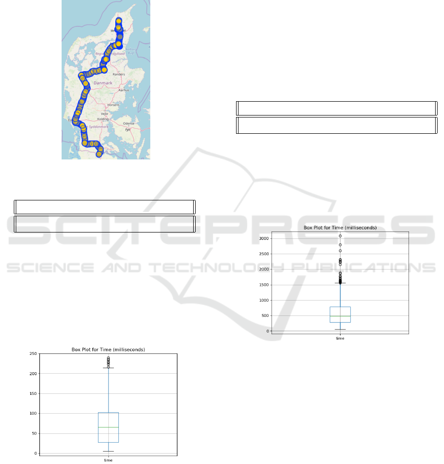
at (57.4468, 10.0260) and the end one at (54.8196,
9.3314) for a distance of approx. 295 km. Routing
between these two towers takes only 0.1587 seconds.
Even when we use the graph without pruning with the
same start and end locations it takes 0.374 second,
which is still quite acceptable.
Figure 6: Routing through Denmark.
Table 3: Routing value for 1000 random samples.
Min Max AVG Median STD
4.92 238.99 73.32 65.31 53.85
Table 3 shows the minimum time (Min), the maxi-
mum time (Max), the average time (AVG), the median
time (Median) and the standard deviation (STD) for
1,000 randomly select pairs of power towers in Den-
mark. Time in this table is in milliseconds rather than
seconds.
Fig. 7 shows a box plot for these routing times of
randomly selected pairs power towers in Denmark.
Figure 7: Box plot of 1000 routings for Denmark.
To summarize, the transformation algorithm is
able to route between tower powers in Denmark in
less than one second – and often in less than 100 mil-
liseconds.
In the next subsection, we analyze France as a use
case for measuring the routing time for a larger grid
by using the transformation algorithm for 1,000 ran-
domly selected routes.
5 EMPIRICAL EVALUATION
(FRANCE)
In this section, we used the transformation algorithm
for routing between randomly selected power towers
in France. We measured the routing time for 1,000
random pairs of power towers.
Table 4: Routing value for 1000 random sample for France.
Min Max AVG Median STD
51.29 3076.86 591.09 480.34 435.14
Table 4 shows minimum time (Min), the maxi-
mum time (Max), the average time (AVG), the median
time (Median) and the standard deviation (STD) in
milliseconds. Fig. 8 shows a box plot for the routing
times between these randomly select power towers in
France.
Figure 8: Box plox of 1000 routings for France.
To summarize, the performance of the transform
algorithm is still very acceptable for larger power
grids. The majority of routes takes less than one sec-
ond.
In the next section, we analyze Europe as a use
case measuring the searching performance of the
transformation algorithm.
6 EMPIRICAL EVALUATION
(EUROPE)
In this section, we measure the performance of the
transformation algorithm for all European countries.
In order to do that we need to follow steps bellow:
GISTAM 2020 - 6th International Conference on Geographical Information Systems Theory, Applications and Management
334
1. Pre-fill caches for all countries
2. Extract the graph from pre-filled caches for all
countries
3. Merge graphs of all countries into a single graph
4. Use transformation algorithm for randomly se-
lected pairs of power towers in Europe countries
Note in particular step 3), where in order to use
the graph for routing by using the transformation al-
gorithm, we have to merge the graphs of all countries
into a single graph. In order to do that, we create
a new graph containing all the edges from the indi-
vidual country graphs. When building the country
graphs, border-crossing power lines were kept in or-
der to facilitate this process.
The code below shows how to merge graphs from
different countries into a single graph.
for country in countries:
for n1, n2, w in country.edges(data=True):
g_merge.add_edge(n1,n2,**data)
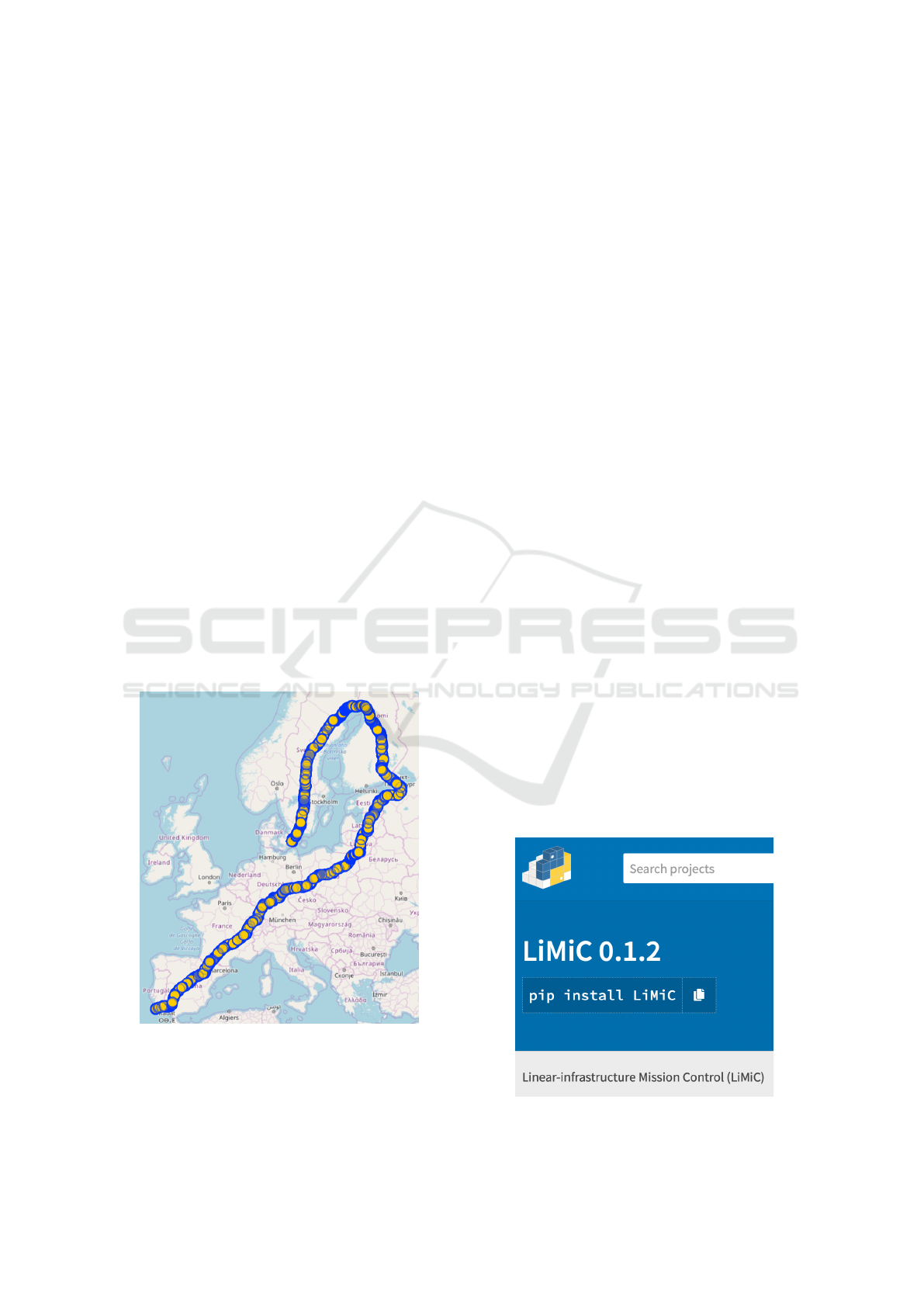
As an example of using the transformation algo-
rithm for routing in the European countries, we have
set (37.1058271, -8.6962473) as the starting location
and (55.4316748, 12.9769681) as the end location.
Fig. 9 shows the outcome of routing algorithm com-
puted in 28.38 seconds. The distance between the
start location and the end location is 2,609.34 km.
The total flying distance along the infrastructure is
6,951,307.18 km.
Figure 9: Routing through European countries.
7 CONCLUSIONS
In this paper, we have developed two routing algo-
rithms for path planing of drone inspections along
linear infrastructures: a direct algorithm and a trans-
formation algorithm. We have shown that the trans-
formation algorithm provides typical sub-second per-
formance even on medium to long distances in large
power grids such as the one of France.
More importantly, the more than satisfactory per-
formance on short distances allows to use this routing
algorithm as an ingredient in optimal mission plan-
ning, where routing can be used to determine the
shortest distances between a number of inspection tar-
gets.
Future work could be to speed up the generation
of the graphs by creating them directly from Open-
StreetMap data. In principle, one could also go be-
yond A*-like algorithms, e.g. investigating the appli-
cability of reach algorithms (Goldberg et al., 2006).
With the level of performance demonstrated and the
typically rather short distance in real-world use cases,
this does not seem necessary, though.
8 OPEN-SOURCE AVAILABILITY
FOR RELEVANCE AND
REPRODUCIBILITY
In order to experiments to be reproducible, we pack-
aged all results described in this paper as a Python
package. The LiMiC (Linear-infrastructure Mission
Control) package is available through The Python
Package Index (PyPI) and can be installed either us-
ing the Package Installer for Python (PIP) by the com-
mand pip install LiMiC or by direct download
from the PyPI: https://pypi.org/project/LiMiC/
Figure 10: LiMiC on the PyPI.
Optimal Path Planning for Drone Inspections of Linear Infrastructures
335

The LiMiC package also also allows other re-
searchers, drone companies, and drone enthusiasts to
build upon the results described in this paper.
ACKNOWLEDGEMENTS
The research leading to these results has re-
ceived funding from the Innovation Fund Denmark
Grand Solutions grant 8057-00038A Drones4Energy
project.
https://drones4energy.dk/.
REFERENCES
Dechter, R. and Pearl, J. (1985). Generalized best-first
search strategies and the optimality of a*. J. ACM,
32(3):505–536.
Ducho
ˇ
n, F., Babinec, A., Kajan, M., Be
ˇ
no, P., Florek, M.,
Fico, T., and Juri
ˇ
sica, L. (2014). Path planning with
modified a star algorithm for a mobile robot. Procedia
Engineering, 96.
Fang, S. X., O’Young, S., and Rolland, L. (2018). Devel-
opment of small uas beyond-visual-line-of-sight (bv-
los) flight operations: System requirements and pro-
cedures. Drones, 2(2).
Goldberg, A., Kaplan, H., and Werneck, R. (2006). Reach
for a*: Efficient point-to-point shortest path algo-
rithms. Technical Report MSR-TR-2005-132, drone.
Technical Report for CLASSiC FP7 European project.
graph tool. Efficent network analysis. Available: https:
//graph-tool.skewed.de/.
Hougardy, S. (2010). The floyd–warshall algorithm on
graphs with negative cycles. Information Processing
Letters, 110(8):279 – 281.
Huber Stephan, R. C. (2016/06/01). Calculate travel time
and distance with openstreetmap data using the open
source routing machine (osrm). SAGE Publications,
2(2).
(Mrs.), E. S. The cost of blackouts in europe. Avail-
able: https://cordis.europa.eu/article/id/126674-the-
cost-of-blackouts-in-europe/.
Nguyen, V. N., Jenssen, R., and Roverso, D. (2019). Intelli-
gent monitoring and inspection of power line compo-
nents powered by uavs and deep learning. IEEE Power
and Energy Technology Systems Journal, 6(1):11–21.
Noto, M. and Sato, H. (2000). A method for the short-
est path search by extended dijkstra algorithm. In
Smc 2000 conference proceedings. 2000 ieee interna-
tional conference on systems, man and cybernetics.
’cybernetics evolving to systems, humans, organiza-
tions, and their complex interactions’ (cat. no.0, vol-
ume 3, pages 2316–2320 vol.3.
python library. dog.pil.core. Available: https://pypi.org/
project/dogpile.core//.
Sathyaraj, B. Moses, J. L. C. F. A. D. S. (2008). Multiple
uavs path planning algorithms: a comparative study.
In Fuzzy Optimization and Decision Making.
University of Southern Denmark, Marianne Harbo Fred-
eriksen, O. V. M. . M. P. K. Drones for inspection of
infrastructure: Barriers, opportunities and success-
ful uses. Available: https://uasdenmark.dk/wp-
content/uploads/2019/06/Final Infrastructure-
Memo 30.05.2019.pdf/.
world, E. Utilities in europe to use long-distance drones to
inspect transmission liness. Available: https://energy.
economictimes.indiatimes.com/news/power/utilities-
in-europe-to-use-long-distance-drones-to-inspect-
transmission-lines/65007676?redirect=1.
GISTAM 2020 - 6th International Conference on Geographical Information Systems Theory, Applications and Management
336
