The Computation of the Inverse Kinematics of a 3 DOF Redundant

Manipulator via an ANN Approach and a Virtual Function

Shahnaz Habibkhah

and Rene V. Mayorga

Department of Industrial Systems Engineering, University of Regina, Regina, SK, Canada

Keywords: Artificial Neural Network, Redundant Robotic Manipulators, Inverse Kinematics.

Abstract: In this paper a method based on Artificial Neural Networks (ANNs) is presented to solve the Inverse

Kinematics (IK) of 3 degrees of freedom (DOF) redundant manipulators. In order to obtain the manipulator’s

joint angles coordinates and solve the IK problem with acceptable accuracy; the forward kinematics equations

of the manipulator are used to obtain position of the end effector, and also a virtual auxiliary function is

included in the ANN approach. Then, the trained ANN’ ability to track a designed target trajectory is tested

inside the workspace of the manipulator in two scenarios with different inputs data to the ANN.

1 INTRODUCTION

The study of robot manipulators motion without

considering the imposed forces is called Forward

Kinematics (FK) (Wang & Chen, 1991, and Murray

et al., 2017). In the FK of a robot manipulator, in

order to obtain the position coordinates of the end-

effector, the robot joint angles are specified.

Whereas, obtaining the joint angles of a robotic

manipulator from Cartesian coordinates of the end

effector is called the Inverse Kinematics (IK) problem

(Wang & Chen, 1991). The IK problem has been very

important as the robot complexity increases, since

obtaining a solution for IK becomes difficult

(Alavandar & Nigam, 2008, and Daya et al., 2010).

This issue is more difficult for redundant

manipulators (RM) (Fu et al., 2013).

The RM is a kind of manipulator in which the

number of DOF is more than what is needed to

perform a task (Chirikjian, 1992, and Sciavicco &

Siciliano, 1988). For this kind of manipulators,

normally there is no direct solution to obtain IK.

Over the years, many numerical and non-

numerical solutions have been proposed to solve IK

of non-RMs and RMs. Aiming to solve the IK of

manipulators, (Oh et al., 1984) has presented a

Newton-Raphson numerical method. The Oh’s paper

has considered a 7 DOF RM as the case study and has

https://orcid.org/0000-0002-3138-7928

https://orcid.org/0000-0001-8365-6571

taken the position coordinates of all links, as well as

the orientation of the end effector into account, as the

constraints. (Gómez et al., 2015) has combined

geometric and numerical ideas to present a solution

for IK. In order to solve IK of RM, (Sciavicco &

Siciliano, 1988) have applied some constraints related

to joint limitations and obstacle avoidance, and a

numerical solution is proposed. Another solution to

the IK of 7 DOF RM is proposed by (Zhao et al.,

2018) where the Newton-Raphson iteration approach

is combined with a damped least square method.

(Zhao et al., 2016) has presented another solution for

the IK of Hyper RM (HRM), in which a new

geometrical method is used. A regression solution has

been also proposed by (Sariyildiz, et al., 2012) to

solve IK of a 7 DOF RM. In this case seven separate

support vector regressions (SVR) are used to solve

the problem since the SVR structure is multi input

single output. However, the SVR solution failed to

solve IK problem of redundant manipulators in the

study proposed by (Bocsi, et al., 2011).

Another approach to solve IK of manipulators is

using non-conventional tools. The idea of using

Fuzzy logic to solve IK is presented by (Howard &

Zilouchian, 1998, and Palm, 1992, and Xu &

Nechyba, 1993). (Palm, 1992) has used this tool to

solve the IK of RMs and a 4 DOF is considered as

case study. Whereas, (Xu & Nechyba, 1993) has used

this tool to solve the IK for both RM and non-RM.

Habibkhah, S. and Mayorga, R.

The Computation of the Inverse Kinematics of a 3 DOF Redundant Manipulator via an ANN Approach and a Virtual Function.

DOI: 10.5220/0009834904710477

In Proceedings of the 17th International Conference on Informatics in Control, Automation and Robotics (ICINCO 2020), pages 471-477

ISBN: 978-989-758-442-8

471

Using Adaptive Neuro-Fuzzy Inference System

(ANFIS), is another idea proposed by (Mohammed

Jasim, 2011). To solve the IK of 2 DOF and 3 DOF

manipulators, (Alavandar & Nigam, 2008) have used

ANFIS. In the paper, in order to provide training data

for ANFIS of 2 DOF manipulator, positions of end

effector are used, and data to train ANFIS of 3 DOF

manipulator is obtained from end effector positions

coordinates and summation of joint angles. Similarly,

(Duka, 2015) has used the end effector positions and

summation of joint angles to train ANFIS to solve the

IK of 3 DOF manipulators.

Some authors have also used ANN to solve the IK

of manipulators. (Duka, 2014) has used ANN to solve

IK of 3 DOF RM in which position coordinates of the

end effector and summation of joint angles are

training inputs. This tool is used to solve IK of a 6

DOF manipulator by (Almusawi et al., 2016) and

training inputs are the end effector desired positions

and orientations as well as current joint angles’

feedback. The paper presented by (El-Sherbiny et al.,

2018) has compared the application of ANN, ANFIS

and Genetic Algorithms methods to solve IK of a 5

DOF manipulator. According to paper’s claims, the

ANN and ANFIS yield the best results. (Thuruthel et

al., 2016) has proposed a solution to solve the inverse

statistics (IS) of redundant soft robots; according to

this study, the inverse statistics is analogous to IK for

rigid robots; thence, many approaches used to solve

IK problem of rigid RM can be utilized to solve the

IS. In their solution, Artificial Neural networks are

used for mapping purposes and the training method is

the Bayesian regularization method (Foresee at al.,

1997).

In this paper, an ANN is used to solve IK problem

of 3 DOF RMs. In order to prepare data to train ANN,

joint angles values are selected randomly and are put

in FK equations of the manipulator and the end

effector’s position as well as its orientation are set as

input data. The orientation of the end effector is

defined according to (Nakamura, 1990) which is

equal to the function cos of the summation of the joint

angles. To evaluate the ANN performance to track a

target trajectory inside the workspace of the

manipulator, the coordinates of the end effector as

well as its expected orientations are applied as the

inputs of ANN. For this purpose, two different

scenarios are considered; in the first case it is assumed

that the end effector should orient in parallel to the

line connected from the end effector to the origin, and

in the second case it is assumed that the end effector

is supposed to orient in parallel to the y axis.

The remainder of this paper is organized as

follows: Section 2 describes the robot manipulator

kinematics equations and end effector workspace.

The Section 3 explains the ANN, and the Section 4

presents the simulation results of the ANN training

and tracking performance of the ANN in 2 scenarios.

Finally, section 5 contains some Conclusions.

2 PROBLEM DESCRIPTION

2.1 Redundant Robot Manipulator

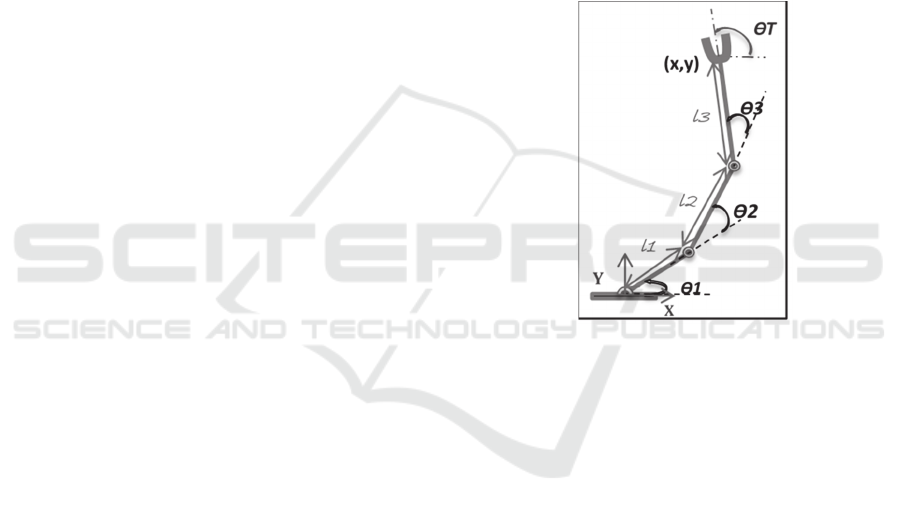
Fig. 1 shows the 3 DOF redundant manipulator (RM)

considered in this paper. To calculate the

manipulator’s end-effector position using the joint

angles, the FK equations are considered.

Figure 1: 3 DOF Redundant Robot Manipulator.

According to the FK equations, the Cartesian

coordinates of the end effector are:

𝑋𝑙1𝑐𝑜𝑠



𝜃1



𝑙2𝑐𝑜𝑠



𝜃1  𝜃2



𝑙3𝑐𝑜𝑠



𝜃1  𝜃2  𝜃3



)

𝑌  𝑙1 𝑠𝑖𝑛𝜃1  𝑙2 𝑠𝑖𝑛



𝜃1  𝜃2



𝑙3𝑠𝑖𝑛



𝜃1  𝜃2  𝜃3



)

Where ɵ

, ɵ

, and ɵ

are the first, second and third

joint angles of the manipulator, and l1, l2 and l3 are

the lengths of the robot arms.

On the other hand, it is impossible to find a unique

set of joint angles of the manipulator from the end

effector’s position coordinates. Normally, an infinite

set of solutions exist. However, an effective approach

as proposed here to deal with this problem, is to

consider a constraint as an auxiliary virtual function

that helps to set a unique solution. It is important to

mention here, that many auxiliary virtual functions

are possible. In fact, a careful selection of the virtual

ICINCO 2020 - 17th International Conference on Informatics in Control, Automation and Robotics

472

auxiliary function may yield an explicit solution to

the IK problem.

Here, as a particular case, the auxiliary virtual

function is selected to represent the end effector’s

orientation. In this paper, the orientation of the end

effector is defined according to (Nakamura, 1990),

which is equal to cos of the summation of the joint

angles as defined next:

𝐶: 𝑐𝑜𝑠



𝜃1  𝜃2  𝜃3



𝑐𝑜𝑠 𝜃𝑇

(3)

Where ɵ

is summation of three joint angles. The

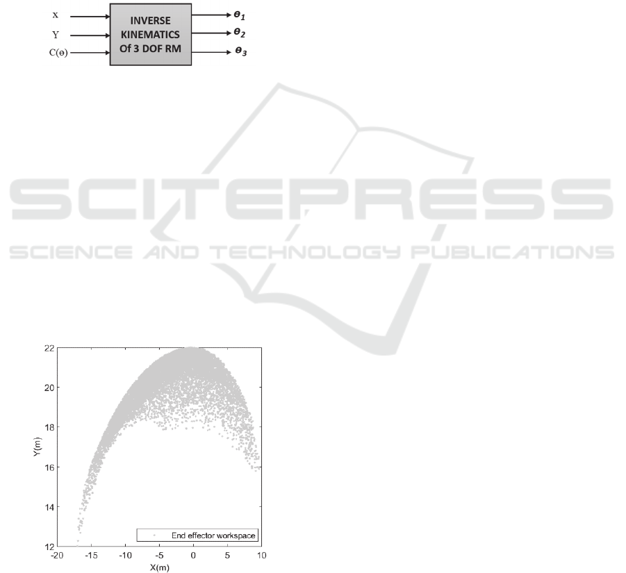
idea of solving IK is depicted in Figure 2; where C(θ)

can be a general case.

Figure 2: Inverse Kinematics Proposed Approach.

2.2 The End Effector Workspace

In order to get a manipulator’s workspace, the length

of the three links as well as the joint angles ranges

should be specified. Changing the joint angles and

feeding them into the FK equations leads to find the

robot’s end effector’s positions and workspace.

Assuming l1=10, l2=7, l3=5, and limiting the angles

inside the ranges mentioned in (4), the end effector’s

positions and workspace of the manipulator will be as

in Figure 3.

𝜋/2  𝜃1  3𝜋/4,  𝜋/4  𝜃2  0 𝑎𝑛𝑑  𝜋/4

𝜃3𝜋/4

(4)

Figure 3: End-effector’s workspace.

3 ANN DESCRIPTION

3.1 ANN Structure

The ANN used in this paper is an adaptive network.

A feedforward network contains some nodes that are

connected by some links together to make

relationships between the nodes. The network takes

some income signals, performs node functions on

signals and generate the outputs (Jang et al., 1997).

An important point about the ANN is that it is able to

update the nodes’ parameters to minimize the error.

Aiming to have an effective ANN, a training

function is needed. A popular training function in

MATLAB is trainlm function which updates bias and

weights using Levenberg-Marquardt (LM)

optimization method. Although this method needs

more memory than other methods; it is the fastest

backpropagation algorithm and is the first choice in

MATLAB (MATLAB, 2018). In this algorithm, in

the first step, some initial random values are assumed

for the weights and the total error is evaluated. Then,

the weights are updated by using a Jacobian matrix

which contains the derivatives of errors with respect

to the weights and biases. Finally, the total error is

updated with respect to the new weights; and based

on the error changes (increment or decrement), the

algorithm switches to other algorithms. The process

will stop once the error amount is smaller than the

required value. Indeed, this algorithm switches to the

steepest descent (also known error backpropagation)

algorithm (Rumelhart et al., 1986) when the curvature

area is complex; and when the local curvature is

quadratic, it switches to the Gauss-Newton (GN)

algorithm to be computationally faster. Still, the LM

is more robust since it can converge if the error

surface is very complex (Yu & Wilamowski, 2011).

3.2 Data Preparation for ANN Design

In order to generate data sets to train the ANN, the

joint angles are feed in (1)-(3) and related end

positions and orientations are obtained. In order to do

this, 10000 random samples for each angle are created

from which 7000 are used for training; 1500 are used

for testing; and 1500 are used for validation. The

inputs of the ANN are these data sets and outputs will

be the joint angles.

The Computation of the Inverse Kinematics of a 3 DOF Redundant Manipulator via an ANN Approach and a Virtual Function

473

4 SIMULATIONS

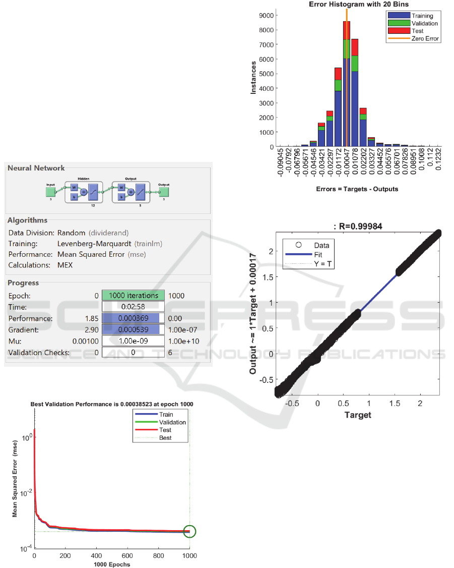
In this section, an ANN with 12 hidden layers is

trained, providing training data mentioned in the last

section, and the training results are depicted. Then

target trajectories are designed inside the workspace

and the ANN ability to track them is considered.

4.1 ANN Design Simulation

Here the ANN training, its performance, error

histogram, and scatter plot of data points’ fit are

shown respectively.

Figure 4: ANN training.

Figure 5: ANN Performance.

Figure 6: ANN Error Histogram.

Figure 7: Scatter plot of data points’ fit.

4.2 Target Trajectory Tracking

The target trajectory is defined by the following

equation and is depicted in Figure 8.

𝑡  65°: 120°, 𝑥  1  16.5 cos



𝑡



,𝑦

 5  16.5sin 𝑡

)

Where x and y are the coordinates of the trajectory

points. In the following subsection, the data

provision for ANN is discussed and the ANN tracking

performance is considered for two cases scenarios.

ICINCO 2020 - 17th International Conference on Informatics in Control, Automation and Robotics

474

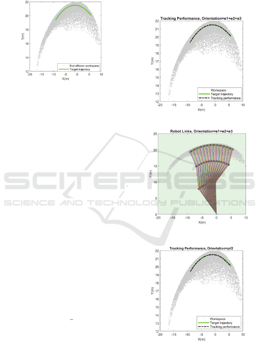
Figure 8: Target trajectory inside the workspace.

4.2.1 First Case Scenario

Regarding to Figure 2, three inputs data are needed

for the ANN inputs. Two of them are the coordinates

of the trajectory points; and the third one should

provide orientation of the end effector as in Eq.(3). In

order to provide data for orientation related to the

points of the target trajectory, in the first case,

orientations of the robot’s end effector are built using

end effector coordinates and is assumed cos(atan2(y,

x)) which means the direction of a line connected

from the end effector to the base of the robot as origin.

Hence, the coordinates of the trajectory points and the

amounts of cos(atan2(y, x)) are inputs of the ANN:

𝑖𝑛𝑝𝑢𝑡𝑠1: 𝑥, 𝑦, cos 𝑎𝑡𝑎𝑛2



𝑥 , 𝑦



]

(6)

The tracking performance of ANN is illustrated in

Figure 9 and the manipulator links status during the

tracking act are shown in Figure 10. As the Figure 10

illustrates, the end effector of the manipulator at each

point is directing toward the origin.

4.2.2 Second Case Scenario

In this scenario, in order to provide data for

orientation related to the points of the target

trajectory, the orientation of the robot end effector is

assumed vertical, which means parallel to the

direction of y-axis, or perpendicular to the x-axis.

Hence the coordinates of the trajectory points and

zero digit (cos(90

)) are inputs of the ANN since :

𝑖𝑛𝑝𝑢𝑡𝑠2: 𝑥, 𝑦, cos 





]

(7)

The tracking performance of ANN is illustrated in

Figure 11 and the manipulator links status during the

tracking act are shown in Figure 12. As the Figure 12

illustrates, the end effector of the manipulator at each

point is directing perpendicular to the x-axis.

Figure 9: Tracking performance of first scenario.

Figure 10: Manipulators links status in first scenario.

Figure 11: Tracking performance of second scenario.

The Computation of the Inverse Kinematics of a 3 DOF Redundant Manipulator via an ANN Approach and a Virtual Function

475

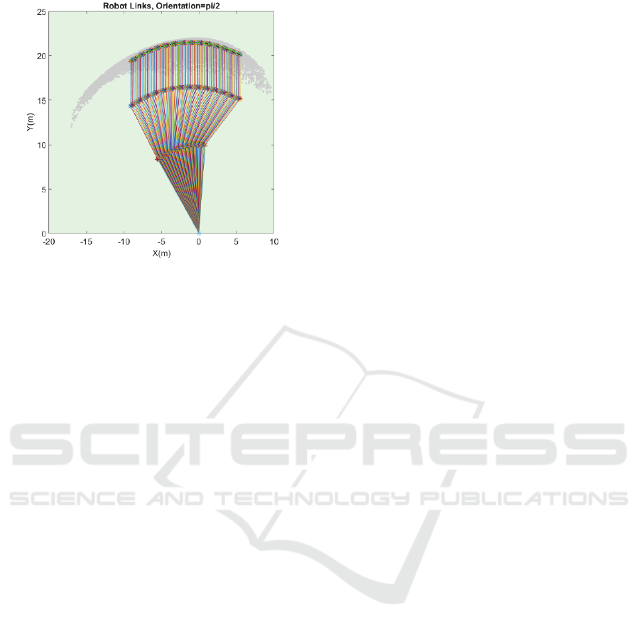
Figure 12: Manipulators links status in second scenario.

As observed at the top portion of the concave

curve in the Figure 12, the proposed approach can

deal with joint configurations close to singularities

(the manipulator fully stretched) without losing

accuracy in the trajectory tracking. This is due to the

auxiliary virtual function acting also as a constraint

(Mayorga, Carrera, 2007) for the singularities

prevention.

5 CONCLUSIONS

In this paper a method based on an Artificial Neural

Network (ANN) approach is presented to solve the IK

of 3 degrees of freedom (DOF) redundant

manipulators. To train the ANN, different joint angles

are feed into the forward kinematics of the

manipulator. Then, the coordinates of the end

effector, and also a virtual function that includes their

orientation are used to provide input data for training

an ANN model that gives as output the joint angles.

According to the ANN training results including

performance and error histogram, the designed ANN

model is satisfactory.

The trained ANN’s ability to track a designed

target trajectory inside the workspace of the

manipulator is tested in two scenarios with different

target orientation of the end effector’s points. In both

cases, the training performance is accurate.

Since the relationship between the inputs and

outputs is nonlinear, the proposed ANN approach is

an efficient solution for this problem compared to

other methods. Moreover, the proposed solution here

is suitable when the purpose is tracking some position

coordinates when one or more constraints exist. In

these cases, finding numerical solutions might be

complex and time-consuming. However, in the

proposed approach, the constraints can be easily

included as virtual functions.

REFERENCES

Alavandar, S., & Nigam, M. J. (2008). Inverse kinematics

solution of 3DOF planar robot using ANFIS. Int. J. of

Computers, Communications & Control, 3, 150-155.

Alavandar, S., & Nigam, M. J. (2008). Neuro-Fuzzy based

Approach for Inverse Kinematics Solution of Industrial

Robot Manipulators. International Journal of

Computers Communications & Control, 3(3), 224.

Almusawi, A. R., Dülger, L. C., & Kapucu, S. (2016). A

New Artificial Neural Network Approach in Solving

Inverse Kinematics of Robotic Arm (Denso VP6242).

Computational Intelligence and Neuroscience, 2016, 1-

10.

Bócsi, B., Nguyen-Tuong, D., Csató, L., Schoelkopf, B., &

Peters, J. (2011, September). Learning inverse

kinematics with structured prediction. In 2011

IEEE/RSJ International Conference on Intelligent

Robots and Systems (pp. 698-703). IEEE.

Chirikjian, G. S. (1992). Theory and applications of hyper-

redundant robotic manipulators (Doctoral dissertation,

California Institute of Technology).

Daya, B., Khawandi, S., & Akoum, M. (2010). Applying

Neural Network Architecture for Inverse Kinematics

Problem in Robotics. Journal of Software Engineering

and Applications, 03(03), 230-239.

Duka, A. (2014). Neural Network based Inverse Kinematics

Solution for Trajectory Tracking of a Robotic Arm.

Procedia Technology, 12, 20-27.

Duka, A. (2015). ANFIS Based Solution to the Inverse

Kinematics of a 3DOF Planar Manipulator. Procedia

Technology, 19, 526-533.

El-Sherbiny, A., Elhosseini, M. A., & Haikal, A. Y. (2018).

A comparative study of soft computing methods to

solve inverse kinematics problem. Ain Shams

Engineering Journal, 9(4), 2535-2548.

Fu, Z., Yang, W., & Yang, Z. (2013). Solution of Inverse

Kinematics for 6R Robot Manipulators With Offset

Wrist Based on Geometric Algebra. Journal of

Mechanisms and Robotics, 5(3).

Foresee, F. D., Hagan, M. T., 1997. Gauss-Newton

approximation to Bayesian regularization. In Proc.

1997 International Joint Conference on Neural

Networks, 1930–1935.

Gómez, S., Sánchez, G., Zarama, J., Ramos, M. C.,

Alcántar, J. E., Torres, J., ... & Lopez, J. A. (2015).

Design of a 4-DOF robot manipulator with optimized

algorithm for inverse kinematics. International Journal

of Mechanical and Mechatronics Engineering, 9(6),

929-934.

Howard, D. W., & Zilouchian, A. (1998). Application of

fuzzy logic for the solution of inverse kinematics and

hierarchical controls of robotic manipulators. Journal of

Intelligent and Robotic Systems, 23(2/4), 217-247.

ICINCO 2020 - 17th International Conference on Informatics in Control, Automation and Robotics

476

Jang, J., Sun, C., & Mizutani, E. (1997). Neuro-Fuzzy and

Soft Computing-A Computational Approach to

Learning and Machine Intelligence [Book Review].

IEEE Transactions on Automatic Control, 42(10),

1482-1484.

MATLAB and Statistics Toolbox Release 2018a, The

MathWorks, Inc., Natick, Massachusetts, United States.

Mayorga, R. V., Carrera, J. (2007). A Radial Basis Network

Approach for the Computation of Inverse Continuous

Time Variant Functions. International Journal of Neural

Systems 17 (03), 149-160.

Mohammed Jasim, W. (2011). Solution of Inverse

Kinematics for SCARA Manipulator Using Adaptive

Neuro-Fuzzy Network. International Journal on Soft

Computing, 2(4), 59-66.

Murray, R. M., Li, Z., & Sastry, S. S. (2017). A

Mathematical Introduction to Robotic Manipulation.

Nakamura, Y. (1990). Advanced robotics: redundancy and

optimization. Addison-Wesley Longman Publishing

Co., Inc..

Oh, S., Orin, D., & Bach, M. (1984). An inverse kinematic

solution for kinematically redundant robot

manipulators. Journal of Robotic Systems, 1(3), 235-

249.

Palm, R. (1992). Control of a redundant manipulator using

fuzzy rules. Fuzzy Sets and Systems, 45(3), 279-298.

Rumelhart, D. E., Hinton, G. E., & Williams, R. J. (1986).

Learning representations by back-propagating errors.

Nature, 323(6088), 533-536.

Sariyildiz, E., Ucak, K., Oke, G., Temeltas, H., & Ohnishi,

K. (2012, July). Support Vector Regression based

inverse kinematic modeling for a 7-DOF redundant

robot arm. In 2012 International Symposium on

Innovations in Intelligent Systems and Applications

(pp. 1-5). IEEE.

Sciavicco, L., & Siciliano, B. (1988). A solution algorithm

to the inverse kinematic problem for redundant

manipulators. IEEE Journal on Robotics and

Automation, 4(4), 403-410.

Thuruthel, T., Falotico, E., Cianchetti, M., Renda, F., &

Laschi, C. (2016, July). Learning global inverse statics

solution for a redundant soft robot.

Wang, L., & Chen, C. (1991). A combined optimization

method for solving the inverse kinematics problems of

mechanical manipulators. IEEE Transactions on

Robotics and Automation, 7(4), 489-499.

Xu, Y., & Nechyba, M. (1993). Fuzzy inverse kinematic

mapping: rule generation, efficiency, and

implementation. Proceedings of 1993 IEEE/RSJ

International Conference on Intelligent Robots and

Systems (IROS '93).

Yu, H., & Wilamowski, B. (2011). Levenberg–Marquardt

Training. Electrical Engineering Handbook, 1-16.

Zhao, J., Xu, T., Fang, Q., Xie, Y., & Zhu, Y. (2018). A

Synthetic Inverse Kinematic Algorithm for 7-DOF

Redundant Manipulator. 2018 IEEE International

Conference on Real-time Computing and Robotics

(RCAR).

Zhao, J., Zhao, L., & Liu, H. (2016). Motion planning of

hyper-redundant manipulators based on ant colony

optimization. 2016 IEEE International Conference on

Robotics and Biomimetics (ROBIO).

The Computation of the Inverse Kinematics of a 3 DOF Redundant Manipulator via an ANN Approach and a Virtual Function

477