Differentially Private Graph Publishing and Randomized Response for
Collaborative Filtering
Juli
´
an Salas
1,2 a
and Vicenc¸ Torra
3,4 b
1
Internet Interdisciplinary Institute (IN3), Universitat Oberta de Catalunya, Barcelona, Spain
2
Center for Cybersecurity Research of Catalonia, Spain
3
Hamilton Institute, Maynooth University, Ireland
4
University of Sk
¨
ovde, Sweden
Keywords:
Noise-graph Addition, Randomized Response, Edge Differential Privacy, Collaborative Filtering.
Abstract:
Several methods for providing edge and node-differential privacy for graphs have been devised. However,
most of them publish graph statistics, not the edge-set of the randomized graph. We present a method for graph
randomization that provides randomized response and allows for publishing differentially private graphs. We
show that this method can be applied to sanitize data to train collaborative filtering algorithms for recom-
mender systems. Our results afford plausible deniability to users in relation to their interests, with a controlled
probability predefined by the user or the data controller. We show in an experiment with Facebook Likes data
and psychodemographic profiles, that the accuracy of the profiling algorithms is preserved even when they are
trained with differentially private data. Finally, we define privacy metrics to compare our method for different
parameters of ε with a k-anonymization method on the MovieLens dataset for movie recommendations.
1 INTRODUCTION
Collaborative filtering algorithms are based on users’
interests to provide recommendations to others. It is
necessary that the users reveal their interests to be able
to build accurate systems, but they may prefer to ex-
clude those that are embarrassing or that reveal their
private preferences. The privacy of users and person-
alization of the algorithms must be balanced.
Statistical techniques have been used for long
time to preserve the privacy of respondents to sur-
veys on social sciences, while preserving the utility of
the responses. Randomized response was devised in
(Warner, 1965) to collect statistical information about
embarrassing or illegal behavior, it provides privacy
by offering plausible deniability for users in relation
to their answers.
It was proved recently that randomized response
is differentially private in (Dwork and Roth, 2014).
Optimal mechanisms for differential privacy by ran-
domized response were calculated in (Wang et al.,
2016; Holohan et al., 2017). Randomized response
was used for protecting privacy for recommendations
a
https://orcid.org/0000-0003-1787-0654
b
https://orcid.org/0000-0002-0368-8037
in (Polat and Du, 2006), however, it was not related to
differential privacy in that setting.
In this paper we present a method for providing
differential privacy in graph publishing with an ap-
plication to collaborative filtering. It is based on the
noise-graph addition technique from (Torra and Salas,
2019) to provide randomized response. By using ran-
domized response, privacy may be enhanced from the
moment of data collection until publication.
This paper is organized as follows. Section 2
presents all the theoretical results for differentially
private graph publication. In Section 3 we present re-
lated work on privacy for collaborative filtering and
present metrics for measuring the privacy provided
when adding noise-graphs. In Section 4 we present
two experiments. The first one shows that precise user
profiles may still be obtained from data with differen-
tial privacy guarantees. The second one, compares the
privacy provided, between different parameter values
and different methods, when collecting data for mak-
ing recommendations. In the last section we present
our conclusions and future work.
Salas, J. and Torra, V.
Differentially Private Graph Publishing and Randomized Response for Collaborative Filtering.
DOI: 10.5220/0009833804150422
In Proceedings of the 17th International Joint Conference on e-Business and Telecommunications (ICETE 2020) - SECRYPT, pages 415-422
ISBN: 978-989-758-446-6
Copyright
c
 2020 by SCITEPRESS – Science and Technology Publications, Lda. All rights reserved
415

2 DIFFERENTIALLY PRIVATE
GRAPH PUBLICATION
In this section we present the noise-graph mechanism
for differentially private graph publication. We pro-
vide the definition of the noise-graph addition tech-
nique and show that it may be applied to obtain ran-
domized response and differential privacy. Finally,
we adapt it to weighted graphs for an application to
user-ratings data for recommender systems.
2.1 Background and Basic Definitions
When the original graph and the noise-graph have
the same sets of nodes we can simplify the defini-
tion of noise-graph addition from (Torra and Salas,
2019). For this, we use the symmetric difference
E
1
4 E
2
:= (E
1
\ E
2
) ∪ (E
2
\ E
1
) = {e|e ∈ E
1
∧ e /∈
E
2
} ∪ {e|e /∈ E
1
∧ e ∈ E
2
}.
Definition 1. Let G
1
(V,E
1
) and G
2
(V,E
2
) be two
graphs with the same nodes V . The addition of G
1
and G
2
is the graph G = (V,E) where E is defined as
E = {e|e ∈ E
1
4 E
2
}.
We will denote G as
G = G
1
⊕ G
2
.
Definition 2 (Noise-graph Addition). Let G be a
graph, let G a family of random graphs. Then, the
noise-graph addition
˜
G following the distribution G
is obtained by drawing a graph g from G and adding
it to G, that is:
˜
G = G ⊕ g.
The most general random graph models in the lit-
erature are the Erd
¨
os-R
´
enyi and the Gilbert model. It
was proved that they are asymptotically equivalent in
(Aiello et al., 2001).
The Gilbert model is denoted by G(n, p), there are
n nodes and each edge is chosen with probability p.
In contrast, the Erd
¨
os-R
´
enyi model that is denoted by
G(n,e), represents a uniform probability of all graphs
with n nodes and e edges. We use the Gilbert model
G(n, p) throughout this paper.
For bipartite graphs, in which there are two sets
of independent nodes U and V , such that |U| = n and
|V | = m, the Gilbert model is denoted as G (n, m, p).
Each of the n × m possible edges in G(n,m, p) has
probability p. We denote the set of bipartite random
graphs with n + m nodes as G
n,m
. Another possible
way of randomizing graphs is through the application
of a randomized response mechanism for a binary at-
tribute (the existence or absence of an edge).
Definition 3 (Design Matrix for Randomized Re-
sponse). A randomised response mechanism for a bi-
nary attribute as defined in (Warner, 1965) is uniquely
determined by its design matrix:
P =

p
00
p
01
p
10
p
11

(1)
where the entry p
jk
= P(X
i
= k|x
i
= j), and X
i
is the
random output for original variable x
i
.
Therefore, p
00
denotes the probability that the
original value is 0 and the randomized value is 0; p
01
denotes the probability that the original value is 1 and
the published value 0; and so on.
For any graph G, if we take g
1
∈ G(n, p
1
) ∩ G,
g
2
∈ G(n, p
2
) \ G, p
1
= 1 − p
11
and p
2
= 1 − p
00
,
then the randomization mechanism A = G⊕g
1
⊕g
2
is
equivalent to the design matrix from eq. (1). In (Wang
et al., 2016) it was proved that if max{
p
00
p
01
,
p
11
p
10
} ≤ e
ε
then the randomized response mechanism following
the design matrix P from Equation (1) is differentially
private.
Definition 4 (Differential Privacy for Graphs). It is
said that a randomized function A is ε-differentially
private if for all neighboring graphs G and G
0
(i.e., differing on at most one element) and all S ⊆
Range(A), it holds that:
Pr[A(G) ∈ S] ≤ exp(ε) × Pr[A(G
0
) ∈ S].
Differential privacy may be defined considering
that neighboring graphs differ either in one node
and all its incident edges, or that they differ in
only one edge, these are the definitons of node or
edge-differential privacy. We first consider edge-
differential privacy (Hay et al., 2009) as it may be
directly related to randomized response. For node-
differential privacy we will use the definition of node
adjacency from (Blocki et al., 2013).
Definition 5 (Node Adjacency). We say that graphs
G and G
0
are neighbors if there exists a node v
i
such
that G − v
i
= G
0
− v
i
. Where G − v denotes the result
of removing every edge in E(G) that touches v.
In other words, the graph G may be obtained from
G
0
by replacing one node and all its neighbors.
2.2 Noise-graph Mechanism
Using definitions from Section 2.1 we are now ready
to define a differentially private mechanism for graph
publishing.
Definition 6 (Noise-graph Mechanism). We define
A
n,p
to be the randomization mechanism that for a
graph G with n nodes and probability
1
2
< p < 1 out-
puts A
n,p
(G) = E(G ⊕ g) with g ∈ G(n, p).
SECRYPT 2020 - 17th International Conference on Security and Cryptography
416

Note that the noise-graph mechanism may be de-
fined for bipartite graphs as follows.
Definition 7 (Bipartite Noise-Graph Mechanism).
For a bipartite graph G = U,V , such that |U| = n,
|V | = m. We define A
n,m,p
to be the randomization
mechanism that for a given probability
1
2
< p < 1 out-
puts A
n,m,p
(G) = E(G ⊕ g) with g ∈ G(n,m, p).
We are going to show that the noise-graph mech-
anism is edge-differentially private, but all the proofs
hold also for the bipartite noise-graph mechanism.
Theorem 1. The noise-graph mechanism A
n,p
is
ln(
1−p
p
)-edge-differentially private.
Proof. By the definition of G(n, p) all the possi-
ble edges in g have probability p. Hence, by Def-
inition 1 if the edge uv ∈ E(G), it will remain in
E(G ⊕ g) with probability 1 − p. Similarly, if uv 6∈
E(G), uv 6∈ E(G ⊕ g) with probability 1 − p. That is,
Pr[uv ∈ E(G ⊕ g)|uv ∈ E(G)] = 1 − p and Pr[uv 6∈
E(G ⊕ g|uv 6∈ E(G)] = 1 − p.
If the edge uv 6∈ E(G), it will be in E(G ⊕ g)
with probability p and analogously if uv ∈ E(G),
with probability p it will not be in E(G ⊕ g). That
is, Pr[uv ∈ E(G ⊕ g)|uv 6∈ E(G)] = p and Pr[uv 6∈
E(G ⊕ g)|uv ∈ E(G)] = p.
Now, assume that G and G
0
differ in the uv
edge, and recall that A
n,p
(G) = G ⊕ g. In ei-
ther case,
Pr[uv∈E(A
n,p
(G))|uv∈E(G)]
Pr[uv∈E(A
n,p
(G
0
))|uv6∈E(G
0
)]
=
1−p
p
≤ exp(ε)
or
Pr[uv6∈E(A
n,p
(G))|uv6∈E(G)]
Pr[uv6∈E(A
n,p
(G
0
))|uv∈E(G
0
)]
=
1−p
p
≤ exp(ε), which
implies that A
n,p
is ε-edge differentially private, for
ε = ln(
1−p
p
).
The mechanism A
n,p
also provides node-
differential privacy for graphs with n nodes. In the
following theorem we denote by G the graph but also
its edge set. We denote the complement of the size of
an edge set X as X =
n(n−1)
2
− X and the complement
G 4 S as the edges that do not belong to the edge set
G 4 S, which are also
n(n−1)
2
− |G ∪ S|.
Theorem 2. The randomized mechanism A
n,p
is
n × ln(
1−p
p
)-node-differentially private.
Proof. For any node u ∈ U and any subset S of all
the possible edges with n nodes. we denote by X =
|G 4 S|. It holds that Pr[A
n,p
(G) = S] = p
X
(1 − p)
X
,
since all the neighbors of u that are not in S, are in the
noise-graph g with probability p, similarly for those
neighbors that are in S but not in G. While the neigh-
bors that are in G ∩ S or in
G ∪ S, i.e., in G 4 S, with
probability 1 − p do not belong to the noise-graph g.
Equivalently for a neighboring graph G
0
, we
denote by X
0
= |G
0
4 S|. Then Pr[A
n,p
(G
0
) ∈
S] = p
X
0
(1 − p)
X
0
. Therefore, we can calculate
Pr[A
n,p
(G)∈S]
Pr[A
n,p
(G
0
)∈S]
=
p
X
(1−p)
X
p
X
0
(1−p)
X
0
= p
X−X
0
(1 − p)
X−X
0
≤ e
ε
.
Considering that X − X
0
= X
0
− X, we obtain that
the mechanism A
n,p
will be differentially private if
ln((
p
1−p
)
X−X
0
) = (X −X
0
)ln(
p
1−p
) < ε. We can bound
X − X
0
by n since G and G
0
are neighboring graphs,
hence A
n,p
is n × ln(
p
1−p
)-differentially private.
2.3 Noise-graph Addition for Weighted
Graphs
In this section we generalize noise-graph addition to
weighted graphs, this will have applications for data
in which the relations are weighted, such as the users’
ratings in recommender systems.
We consider a weighted graph to be a graph G
with node set V (G), edge set E(G) and a function
ω : E(G) → [0, 1], that to each edge e ∈ V (G) assigns
a weight ω(e) ∈ [0,1]. That is, we are considering
graphs in which the edges have weights between 0
and 1. In some cases this weight can represent the
probability that u and v are connected, or the strength
of their relation. For the case of relations weighted by
ordinal numbers (e.g., t ∈ {0,1, ..., m}) the weights
may be transformed to numbers in [0,1] easily by di-
viding them by the maximum number, i.e.,
t
m
in the
example.
From a mathematical point of view, ⊕ can be un-
derstood as an exclusive or of the existence of the
edges. So, 0 ⊕ 0 = 0, 1 ⊕ 0 = 1, 0 ⊕ 1 = 1, 1 ⊕ 1 = 0,
where 1 and 0 means existence or not of the edge.
Understanding ⊕ from this perspective, we can
exploit fuzzy set theory to define ⊕. Fuzzy set the-
ory provides operations that generalize conjunction
(functions called t-norms and denoted T ), disjunction
(functions called t-conorms and denoted S) and com-
plement (through functions called negations and de-
noted N). These operations are defined on the inter-
val [0,1] or [0,1]
2
instead of being defined on {0,1}
or {0,1}
2
as required by classical set theory and clas-
sical logic. Then, using standard logic properties, we
know that:
x ⊕ y = (x ∨ y)∧ ¬(x ∧ y).
Using this logical equivalence, we can define x ⊕ y
when x ∈ [0,1] and y ∈ [0, 1] in terms of t-norms T , t-
conorms S and negations N. That is,
x ⊕ y = T (S(x,y),N(T (x,y))).
The functions t-norms, t-conorms, and negations
are established according to a set of axioms that gen-
eralize the properties of conjunction (and intersec-
tion), disjunction (and union), and complement. Be-
cause of that there are families of functions for each
Differentially Private Graph Publishing and Randomized Response for Collaborative Filtering
417

of them. For the sake of simplicity, we will use
T (x,y) = min(x, y), S(x, y) = max(x, y) and N(x) =
1 − x. For details and alternatives see e.g., (Klir and
Yuan, 1995). Using these functions, we define ⊕ as
follows:
x ⊕ y = min(max(x,y),1 − min(x,y)).
Definition 8 (Weighted Noise-Graph Addition). Let
G
1
(V,E
1
,ω
1
) and G
2
(V,E
2
,ω
2
) be two graphs with
the same nodes V . We define the addition of G
1
and
G
2
as the graph G = G
1
⊕ G
2
= (V,E,ω) with ω(E)
as follows:
ω(e) = ω
1
(e), for e ∈ E
1
\ E
2
,
ω(e) = ω
2
(e), for e ∈ E
2
\ E
1
,
ω(e) = min(max(ω
1
(e),ω
2
(e)),1 − min(ω
1
(e),ω
2
(e)),
for e ∈ E
1
∪ E
2
.
3 PRIVACY FOR
RECOMMENDER SYSTEMS
In this section we apply the noise-graph mechanism
to bipartite graphs, all the proofs from Section 2.2
are equivalent, by assuming that G is bipartite and
changing A
n,p
(G) for A
n,m,p
(G) defining E(G ⊕ g)
with g ∈ G(n, m, p).
We can represent the user-item graph generated
from the data for recommendations as a bipartite
graph of U users and V items, with an edge e = uv if
the user u ∈ U has liked the item v ∈ V . For numerical
ratings, we may represent them by a weighted graph
in which the weight of an edge ω(e) represents the
rating normalized to [0, 1]. A recommendation may
be formulated as a link prediction problem in such
graphs, or by representing the graphs with their adja-
cency matrix with U as rows and V as columns and us-
ing matrix factorization models (Koren et al., 2009).
Similar methods have been successfully used for pre-
dicting private traits such as sexual, political or reli-
gious preferences from Likes in (Kosinski et al., 2013;
Kosinski et al., 2016).
3.1 Related Work
There are diverse ways to protect users’ privacy, such
as protecting them from precise inference of private
attributes, protecting them from reidentification as in
(Salas, 2019) with k-anonymity, or to afford them
with plausible deniability as in randomized response
mechanisms.
Randomized response was used in (Wang et al.,
2016) for differentially private data-collection, it was
compared to the Laplace mechanism and provided an
empirical evaluation including graph statistics. It was
also used in (Polat and Du, 2006) to protect privacy
for recommendations with binary ratings, however,
they did not consider that differential privacy may be
obtained.
Randomized response and differential privacy
were used in (Liu et al., 2017) to provide privacy dur-
ing the data collection and data publication stages.
They added random uniform noise to the user-ratings
and provided differential privacy for the item-item co-
variance matrix, which was defined in (Mironov and
McSherry, 2009) after the Netflix prize contest de-
anonymization (Narayanan and Shmatikov, 2008).
In (Salas, 2019) the method for differential pri-
vacy from (Mironov and McSherry, 2009) was com-
pared with a method for k-anonymization for recom-
mendations. The concept of k-anonymity was orig-
inally defined for tables (Samarati, 2001), (Sweeney,
2002) and the attributes were classified on the disjoint
classes of Identifiers (IDs), Quasi-Identifiers (QIs),
Sensitive Attributes (SAs) and Non-sensitive.
Some variants and extensions have been provided
for k-anonymity such as ` diversity (Machanavajjhala
et al., 2007) and t-closeness approach (Li et al., 2007),
as well as for ε-differential privacy (Desfontaines
and Pej
´
o, 2019), including (ε, δ)-differential privacy
(Dwork et al., 2006). Some of their differences and
interactions are discussed in (Salas and Domingo-
Ferrer, 2018).
3.2 Privacy Metrics for Adding
Noise-graphs
We devise metrics to measure the privacy provided
by a sanitization method with different parameters,
that will be also useful to compare among different
methods, such as ε-differential privacy, k-anonymity
or any of their variants. First, we provide the defi-
nitions of k-anonymity from (Samarati, 2001) as de-
fined in (Torra, 2017) and Risk and Imprecision mea-
sures from (Salas, 2019).
Definition 9. A dataset is k-anonymous if each record
is indistinguishable from at least other k − 1 records
within the dataset, when considering the values of its
QIs. That is, if we denote the set of QI values of
a record j as Q
j
, then for each record j there are
at least other k − 1 records { j
1
,.. ., j
k−1
} such that
Q
j
i
= Q
j
for all i ∈ {1,.. ., k − 1}.
Definition 10. For each user u the Sensitive Attribute
Risk (SA
R
) of a sanitization is defined as the propor-
tion of her observed records R
u
that are part of her
SECRYPT 2020 - 17th International Conference on Security and Cryptography
418

true records r
u
, that is:
SA
R
(u) =
|r
u
|
|R
u
|
(2)
Note that Definition 10, considers that the pub-
lished data for each user u (observed records R
u
)
contains the true data (r
u
). This equals the Jaccard
similarity J(R
u
,r
u
) =
|R
u
∩r
u
|
|R
u
∪r
u
|
=
|r
u
|
|R
u
|
when r
u
⊂ R
u
.
However, if we consider the Jaccard distance in-
stead, we obtain d
J
(R
u
,r
u
) = 1 − J(R
u
,r
u
) =
R
u
4r
u
R
u
∪r
u
.
In our graph representation user’s u true records
r
u
equal N
G
(u) and R
u
equals N
˜
G
(u), where
˜
G = A
n,p
(G) = G ⊕ g. Hence, 1 − SA
R
(u) =
d
J
(R
u
,r
u
) = d
J
(N
˜
G
(u),N
G
(u)) =
|N
˜
G
(u)4N
G
(u)|
|N
˜
G
(u)
S
N
G
(u)|
=
|N
G
L
g
(u)
L
N
G
(u)|
|N
G
L
g
(u)
S
N
G
(u)|
=
|N
G
(u)
L
N
g
(u)
L
N
G
(u)|
|(N
G
(u)
L
N
g
(u))
S
N
G
(u)|
=
|N
g
(u)|
|N
g
(u)
S
N
G
(u)|
.
This distance may equal 1 if N
˜
G
(u)
T
N
G
(u) =
/
0,
in that case it will be 1 for sets that are quite differ-
ent, hence it will not measure how many changes have
been done to the original set. Therefore, we propose
to use instead d(N
˜
G
(u),N
G
(u)) =
|N
g
(u)|
|N
g
(u)|+|N
G
(u)|
which
will consider the number of modified items in pro-
portion to the number of real items liked by user u.
Consequently, we define the Sensitive Attribute Risk
for any graph as 1 − d(N
˜
G
(u),N
G
(u)) in equation (3)
which is consistent with Definition 10.
Definition 11. Let G be a graph,
˜
G a protected ver-
sion of graph G with the same number of nodes as G.
Let g =
˜
G
L
G the edge difference between
˜
G and G
(i.e., the noise added to G). We define the Sensitive
Attribute Risk for a node u ∈ V (G) as:
SA
R
(u) =
|N
G
(u)|
|N
g
(u)| + |N
G
(u)|
(3)
In the case of weighted graphs Definition 11, is
still relevant since it measures the risk by the num-
ber of movies. However, the weight can be con-
sidered by replacing |N
G
(u)| by its weighted ver-
sion which we will denote as ω(N
G
(u)) and define as
ω(N
G
(u)) =
∑
v∈N
G
(u)
ω(uv). Therefore, we obtain the
following definition, which generalizes previous one,
considering that for an unweighted graph the weight
function ω(uv) = 1 for all uv ∈ E(G) can be used.
Definition 12. Let G be a weighted graph, ω its
weight function,
˜
G a protected version of graph G
with the same number of nodes as G. Let g =
˜
G
L
G
the edge difference between
˜
G and G (i.e., the noise
added to G). We define the Weighted Sensitive At-
tribute Risk for a node u ∈ V (G) as:
SA
R
(u) =
ω(N
G
(u))
ω(N
g
(u)) + ω(N
G
(u))
(4)
Definition 13. Let G be a weighted graph, ω its
weight function,
˜
G a protected version of graph G.
The Average Sensitive Attribute Imprecision (SA
I
) is
defined as follows:
SA
I
=
1
E(G ∪
˜
G)
∑
e∈E(G∪
˜
G)
|ω
˜
G
(e) − ω
G
(e)| (5)
Note that SA
I
is a well known measure for the in-
formation loss, that is the mean average error. How-
ever, when all the attributes are at the same time QIs
and SAs it measures both the disclosure risk and the
information loss.
After defining these metrics, we perform the util-
ity/privacy evaluation in the following section.
4 EXPERIMENTS
In this section we apply our algorithms to data that
was used to predict users’ psychodemographics, as
well as for training collaborative filtering algorithms.
4.1 Facebook Likes Dataset for
Psychodemographic Inference
In this section we will protect Facebook Likes data
from (Kosinski et al., 2016). The dataset con-
sists of Facebook users (110, 728), Facebook Likes
(1,580,284) and their user-likes pairs (10,612,326).
This data was used to predict the pyschodemograph-
ics of the same users, measured by a 100-item long
International Personality Item Pool questionnare mea-
suring the five-factor model of personality (Goldberg
et al., 2006), which are their gender, age, political
views, and their scores on openness, conscientious-
ness, extroversion, agreeableness, and neuroticism.
Since this dataset is sparse there are a large num-
ber of users and items that appear few times, such
data points are of little significance for building a
model to perform inference. We follow the same ap-
proach of trimming the User-Like Matrix to obtain
the same dataset to perform inference as in (Kosinski
et al., 2016). They chose the thresholds of minimum
50 likes per user and 150 users per like, to obtain a
dataset with n = 19,724 users, m = 8,523 likes (POIs)
and q = 3,817,840 user-like pairs.
With this data we will generate a bipartite graph
G of users U, likes L with |U| = n, |L| = m and
|E(G)| = q. Hence, for adding random noise to G we
will sample bipartite random graphs g ∈ G(n, m, p).
We recall that A
n,m,p
(G) is ε-edge differentially
private for ε = ln(
1−p
p
), as we pointed out at the beg-
gining of Section 3. In Table 1 we present the corre-
sponding values and the number of user-likes in the
Differentially Private Graph Publishing and Randomized Response for Collaborative Filtering
419

randomized graph A
n,m,p
(G) = G ⊕ g of our experi-
ments. Note that for each p we obtain noise-graphs g
with p × n ×m = p × 168,107,652 edges on average.
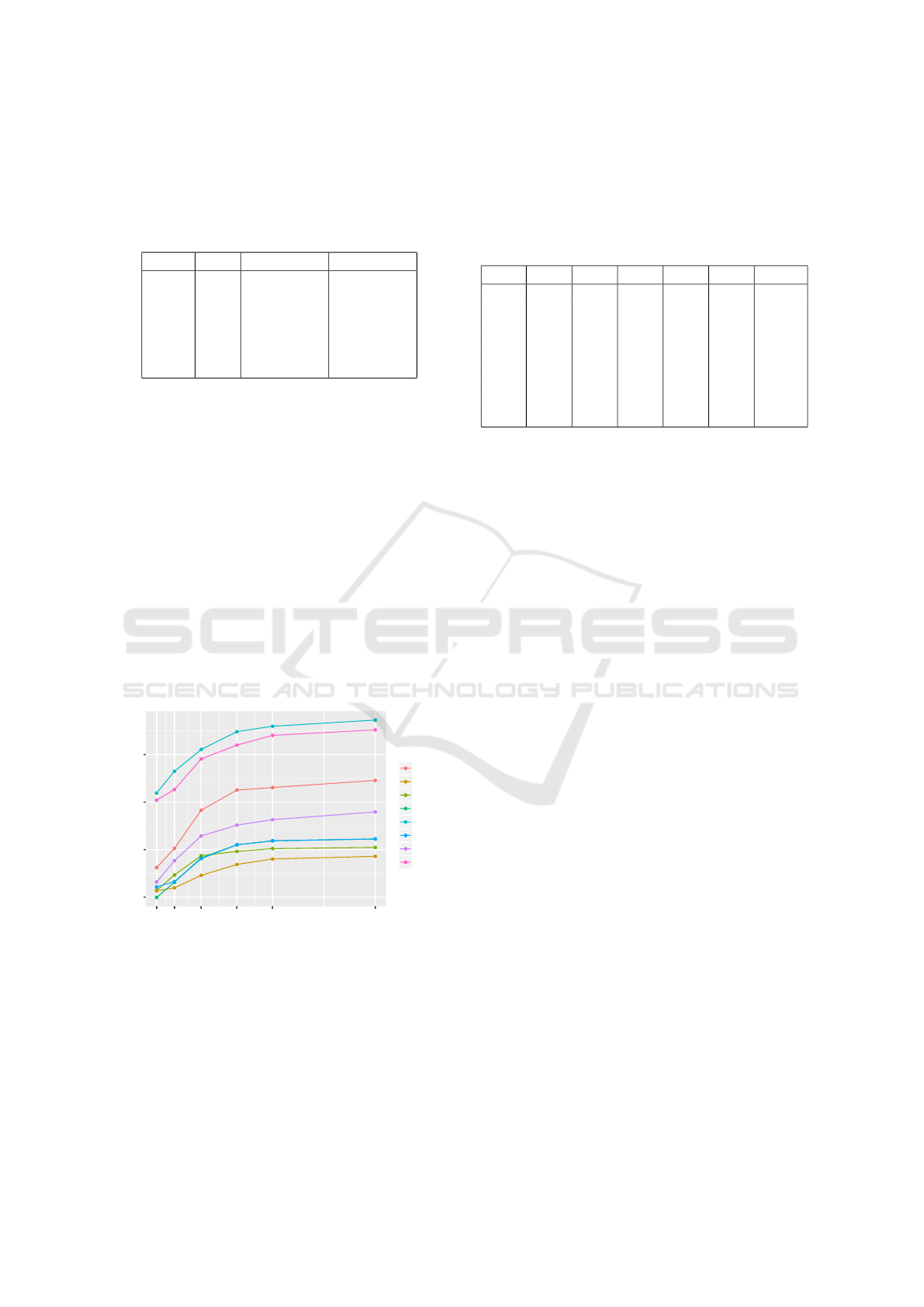
Table 1: Values of p, ε and number of user-likes in the ran-
domized graph.
p ε |E(g)| |E(G ⊕ g)|
0.005 5.29 840,162 4,619,770
0.05 2.94 8,408,449 11,844,981
0.1 2.19 16,824,538 19,878,770
0.2 1.38 33,657,261 35,949,261
0.3 0.84 50,482,636 52,007,684
0.4 0.40 67,302,556 68,070,070
For inference, we performed Singular Value De-
composition (SVD), cf. (Leskovec et al., 2014).
Then, use logistic regression for predicting variables
values (such as gender or political views) from the
user SVD scores in the training subset. We use 10-
fold cross-validation and AUC and Pearson correla-
tion coefficient to measure the accuracy of the predic-
tions following from (Kosinski et al., 2016).
After performing inference on the data repre-
sented by G, we compare with the results for each
of the differentially private graphs A
n,m,p
(G) = G
ε
to measure the accuracy lost when providing privacy
guarantees to the data subjects, see Figure 1. Recall
that the variables are gender, age, political views, and
users’ scores on openness, conscientiousness, extro-
version, agreeableness, and neuroticism.
0.00
0.25
0.50
0.75
5.35.35.35.35.35.35.35.33.03.03.03.03.03.03.03.02.22.22.22.22.22.22.22.21.41.41.41.41.41.41.41.40.80.80.80.80.80.80.80.80.40.40.40.40.40.40.40.4
ε values
Prediction Accuracy
Variable
age
agr
con
ext
gender
neu
ope
political
Figure 1: Accuracy for predictions depending on the ε.
We see in Figure 1, that for probabilities p ≤ 0.1
or equivalently ε ≥ 2.2, the data utility is barely re-
duced. The predictions on demographics remain quite
precise, as we show in Table 2 were the imprecision
is measured (in %) as the proportion of the error be-
tween the obtained precision on the sanitized data
with ε-differential privacy with respect to the origi-
nal precision obtained without sanitizing the dataset.
The values for the accuracy on the data without san-
itization are gender = 0.936, age = 0.616, political =
0.884, openness = 0.450, conscientiousness = 0.264,
extroversion = 0.309, agreeableness = 0.213 and neu-
roticism = 0.304.
Table 2: Imprecision of predictions depending on ε (mea-
sured in %).
att/ε 5.29 2.94 2.19 1.38 0.84 0.40
gen 0.5 4 7 17 29.2 41.5
age 0.4 6.4 8.5 25.8 58.4 74.7
pol 0.5 3.7 9.5 17.7 35.9 42.3
ope 0.3 9.3 15.7 28.3 57.3 82.2
con 0.9 3.2 8.7 17.4 55.8 86.5
ext 0.8 3.9 10.7 33 74.5 100.5
agr 0.9 5.7 19.1 46 76.8 84.2
neu 0.7 2.5 9.4 33.4 72.9 82.2
4.2 MovieLens Dataset for
Collaborative Filtering
In this section we protect the Movielens-100K dataset
(Harper and Konstan, 2015) that is used commonly
as a benchmark dataset for collaborative filtering.
The Movielens-100K dataset contains 100,000 rat-
ings (between 1 and 5) with timestamps that 943 users
gave to 1,682 movies.
With this data we generate a weighted bipartite
graph G of users U and movies V , with the weight
function ω : E(G) → [0,1] such that ω(uv) is the rat-
ing that user u assigned to movie v. For adding noise
to such graph we apply the techniques from Section
2.3, we generate noise-graphs as in Theorems 1 and
2. Additionally we define the weight function for
the noise-graph g to be ω
0
that assigns edge weights
from the empirical distribution of the edge weights
assigned by ω to G, the rationale behind this is that
assigning a constant weight ω
0
= c for all edges in
g may facilitate identifying the noise-edges that have
been added to G. The distribution of the weights of
the edges and the weighted sum function, may play a
key role to prove that the weighted noise-graph addi-
tion is differentially private, we leave such proof for
future work.
We perform a comparison with an algorithm
providing k-anonymity, i.e., HAKR algorithm from
(Salas, 2019). We measure the privacy provided by
both algorithms, to show that even when using two a-
priori different models for privacy protection, we may
still be able to compare their privacy guarantees.
In Table 3 we show the values of p and the num-
ber of ratings (edges) in the noise-graph and the ran-
domized graph. Note that since we consider only the
ratings in the train set the edges of the graph G to be
protected.
SECRYPT 2020 - 17th International Conference on Security and Cryptography
420

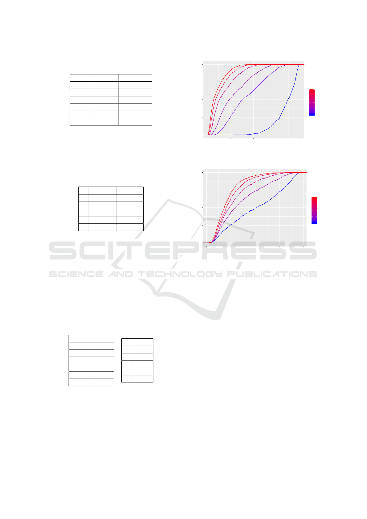
Table 3: Values of p and number of ratings in the random-
ized graph.
p |E(g)| |E(G ⊕ g)|
0.005 7,728 87,354
0.05 77,907 153,864
0.1 155,663 227,698
0.2 312,148 376,192
0.3 466,739 522,564
0.4 621,566 669,706
In Table 4 we consider the noise added to G to ob-
tain the sanitized graph
˜
G as in 11, where g =
˜
G
L
G.
Note that in this case g is not a random graph, and the
graph that is k-anonymized is the graph correspond-
ing to the train set of 80K ratings.
Table 4: Values of k and number of ratings added in the
sanitized graph.
k |E(g)| |E(
˜
G)|
2 74,444 154,444
3 132,236 212,236
4 178,469 258,469
5 214,966 294,966
6 249,806 329,806
In Figures 2 and 3 we plot the cumulative dis-
tributions of the values of the Sensitive Attribute
Risk for all the users. In Figure 2 we see that
the mean values for SA
R
in the randomized data are
0.84,0.42,0.28, 0.18,0.13 and 0.10, respectively, for
p = 0.005,0.05,0.1, 0.2,0.3, 0.4. While in Figure 3
the mean values for SA
R
in the k-anonymous data
are 0.50, 0.35,0.28,0.24,0.21, respectively, for k =
2,3,4, 5,6. The privacy provided not only depends on
the method, but also on the parameter. For example,
for p = 0.1 and k = 4 the average SA
R
is the same.
Table 5: Information loss/disclosure risk measured as aver-
age SA
I
.
p SA
I
0.005 0.3025
0.05 1.732
0.1 2.351
0.2 2.855
0.3 3.080
0.4 3.197
k SA
I
2 1.713
3 2.209
4 2.443
5 2.571
6 2.675
Finally, in Table 5 we compare the Informa-
tion loss (as mean SA
I
) between a priori different
sanitization methods such as adding noise and k-
anonymization. The positive aspect of randomization
is that p is a continuous value, while k is discrete, so
randomization can be better tuned for more specific
privacy and utility values.
0.00
0.25
0.50
0.75
1.00
0.00 0.25 0.50 0.75 1.00
Sensitive Attribute Risk
Cumulative Distribution
0.1
0.2
0.3
0.4
p
Figure 2: Sensitive attribute risk cumulative distribution
grouped by p.
0.00
0.25
0.50
0.75
1.00
0.00 0.25 0.50 0.75 1.00
Sensitive Attribute Risk
Cumulative Distribution
2
3
4
5
6
k
Figure 3: Sensitive attribute risk cumulative distribution
grouped by k.
5 CONCLUSIONS
In this paper, we presented a method for differen-
tially private graph-publishing based on noise-graph
addition. Then, we showed that it may be applied
to obtain randomized response and differential pri-
vacy for collaborative filtering. Finally, we provided a
measure for privacy of a sanitization method, that al-
lows to compare between algorithms with different a-
priori guarantees, such as ε-differential privacy and k-
anonymity. We tested our algorithms in public Face-
book Likes to prove that the accuracy of profiling al-
gorithms is well preserved even when they are trained
with differentially private data. The experiment on
MovieLens dataset shows an application for sanitiz-
ing weighted graphs for recommendations. We can
conclude from our results that is possible to provide
strong privacy guarantees to users, while still obtain-
ing accurate recommendations and predictions. We
leave as future work to show that our method may
provide ε-differential privacy for weighted graphs.
Differentially Private Graph Publishing and Randomized Response for Collaborative Filtering
421

ACKNOWLEDGEMENTS
This work was partially supported by the Swedish Re-
search Council (Vetenskapsr
˚
adet) project DRIAT (VR
2016-03346), the Spanish Government under grants
RTI2018-095094-B-C22 ”CONSENT”, and the UOC
postdoctoral fellowship program.
REFERENCES
Aiello, W., Chung, F., and Lu, L. (2001). A random graph
model for power law graphs. Experimental Mathemat-
ics, 10(1):53–66.
Blocki, J., Blum, A., Datta, A., and Sheffet, O. (2013). Dif-
ferentially private data analysis of social networks via
restricted sensitivity. In Proceedings of the 4th Con-
ference on Innovations in Theoretical Computer Sci-
ence, ITCS ’13, pages 87–96.
Desfontaines, D. and Pej
´
o, B. (2019). Sok: Differential
privacies.
Dwork, C., Kenthapadi, K., McSherry, F., Mironov, I., and
Naor, M. (2006). Our data, ourselves: Privacy via
distributed noise generation. In Vaudenay, S., editor,
Advances in Cryptology - EUROCRYPT 2006, pages
486–503.
Dwork, C. and Roth, A. (2014). The algorithmic foun-
dations of differential privacy. Found. Trends Theor.
Comput. Sci., 9(3—4):211–407.
Goldberg, L. R., Johnson, J. A., Eber, H. W., Hogan,
R., Ashton, M. C., Cloninger, C. R., and Gough,
H. G. (2006). The international personality item pool
and the future of public-domain personality measures.
Journal of Research in Personality, 40(1):84 – 96.
Proceedings of the 2005 Meeting of the Association
of Research in Personality.
Harper, F. M. and Konstan, J. A. (2015). The movielens
datasets: History and context. ACM Trans. Interact.
Intell. Syst., 5(4):19:1–19:19.
Hay, M., Li, C., Miklau, G., and Jensen, D. (2009). Ac-
curate estimation of the degree distribution of private
networks. In 2009 Ninth IEEE International Confer-
ence on Data Mining, pages 169–178.
Holohan, N., Leith, D. J., and Mason, O. (2017). Optimal
differentially private mechanisms for randomised re-
sponse. IEEE Transactions on Information Forensics
and Security, 12(11):2726–2735.
Klir, G. J. and Yuan, B. (1995). Fuzzy Sets and Fuzzy Logic:
Theory and Applications. Prentice-Hall, Inc., USA.
Koren, Y., Bell, R., and Volinsky, C. (2009). Matrix factor-
ization techniques for recommender systems. Com-
puter, 42(8):30–37.
Kosinski, M., Stillwell, D., and Graepel, T. (2013). Pri-
vate traits and attributes are predictable from digital
records of human behavior. Proceedings of the Na-
tional Academy of Sciences, 110(15):5802–5805.
Kosinski, M., Wang, Y., Lakkaraju, H., and Leskovec,
J. (2016). Mining big data to extract patterns and
predict real-life outcomes. Psychological Methods,
21(4):493–506.
Leskovec, J., Rajaraman, A., and Ullman, J. D. (2014). Min-
ing of Massive Datasets. Cambridge University Press,
2 edition.
Li, N., Li, T., and Venkatasubramanian, S. (2007).
t-closeness: Privacy beyond k-anonymity and l-
diversity. In 2007 IEEE 23rd International Confer-
ence on Data Engineering, pages 106–115.
Liu, X., Liu, A., Zhang, X., Li, Z., Liu, G., Zhao, L., and
Zhou, X. (2017). When differential privacy meets ran-
domized perturbation: A hybrid approach for privacy-
preserving recommender system. In Database Sys-
tems for Advanced Applications, pages 576–591.
Machanavajjhala, A., Kifer, D., Gehrke, J., and Venkitasub-
ramaniam, M. (2007). L-diversity: Privacy beyond
k-anonymity. ACM Trans. Knowl. Discov. Data, 1(1).
Mironov, I. and McSherry, F. (2009). Differentially pri-
vate recommender systems: Building privacy into the
netflix prize contenders. In Proceedings of the 15th
ACM SIGKDD International Conference on Knowl-
edge Discovery and Data Mining (KDD), pages 627–
636.
Narayanan, A. and Shmatikov, V. (2008). Robust de-
anonymization of large sparse datasets. In 2008 IEEE
Symposium on Security and Privacy (sp 2008), pages
111–125.
Polat, H. and Du, W. (2006). Achieving private recom-
mendations using randomized response techniques. In
Advances in Knowledge Discovery and Data Mining,
pages 637–646.
Salas, J. (2019). Sanitizing and measuring privacy of large
sparse datasets for recommender systems. Journal of
Ambient Intelligence and Humanized Computing.
Salas, J. and Domingo-Ferrer, J. (2018). Some basics
on privacy techniques, anonymization and their big
data challenges. Mathematics in Computer Science,
12(3):263–274.
Samarati, P. (2001). Protecting respondents identities in mi-
crodata release. IEEE Transactions on Knowledge and
Data Engineering, 13(6):1010–1027.
Sweeney, L. (2002). k-anonymity: A model for protecting
privacy. International Journal of Uncertainty, Fuzzi-
ness and Knowledge-Based Systems, 10(05):557–570.
Torra, V. (2017). Data privacy: Foundations, new develop-
ments and the big data challenge. Springer.
Torra, V. and Salas, J. (2019). Graph perturbation as
noise graph addition: A new perspective for graph
anonymization. In Data Privacy Management, Cryp-
tocurrencies and Blockchain Technology, pages 121–
137.
Wang, Y., Wu, X., and Hu, D. (2016). Using randomized
response for differential privacy preserving data col-
lection. In EDBT/ICDT2016WS.
Warner, S. L. (1965). Randomized response: A survey tech-
nique for eliminating evasive answer bias. Journal of
the American Statistical Association, 60(309):63–69.
SECRYPT 2020 - 17th International Conference on Security and Cryptography
422