
Accelerating Interval Iteration for Expected Rewards in Markov
Decision Processes
Mohammadsadegh Mohagheghi
1 a
and Khayyam Salehi
2 b
1
Department of Computer Science, Vali-e-Asr University of Rafsanjan, Rafsanjan, Iran
2
Department of Computer Science, Shahrekord University, Shahrekord, Iran
Keywords:
Probabilistic Model Checking, Expected Rewards, Markov Decision Processes, Interval Iteration.
Abstract:
Reachability probabilities and expected rewards are two important classes of properties that are computed
in probabilistic model checking. Iterative numerical methods are used to compute these properties. Interval
iteration and sound value iteration are proposed in recent years to guarantee the precision of computed values.
These methods consider upper and lower bounds of values and update each bound in every iteration until
satisfying the convergence criterion. In this paper, we focus on the computation of the expected rewards
of models and propose two heuristics to improve the performance of the interval iteration method. The first
heuristic updates the upper and lower bounds separately to avoid redundant updates. The second heuristic uses
the computed values of the lower bound to approximate a starting point for the upper bound. We also propose
a criterion for the correctness of the approximated upper bound. The experiments show that in most cases,
interval iteration with our approaches outperforms the standard interval iteration and sound value iteration
methods.
1 INTRODUCTION
Probabilistic model checking is widely used for ver-
ification of quantitative and qualitative properties of
stochastic systems. Markov chains and Markov deci-
sion processes (MDPs) are well-known transition sys-
tems that are used to model stochastic and probabilis-
tic systems (Baier and Katoen, 2008). A wide range
of properties that are analyzed in probabilistic model
checking are reduced to the computation of reacha-
bility probabilities and expected rewards (Baier and
Katoen, 2008; Forejt et al., 2011). In reachability
probabilities, the probability of finally reaching a goal
state should be computed. In expected rewards, the
expectation of the accumulated rewards until reach-
ing a goal state is computed. For the case of MDPs,
which are used to model non-deterministic choices of
systems, the extremal (maximal or minimal) reacha-
bility probabilities or expected rewards are considered
(Forejt et al., 2011). Linear programming techniques
or iterative numerical methods can be used for com-
puting these properties. The first class of techniques is
useful for computing the exact values, but is limited
to small models (Forejt et al., 2011; Katoen, 2016;
a
https://orcid.org/0000-0001-8059-3691
b
https://orcid.org/0000-0002-3379-798X
Agha and Palmskog, 2018). Considering finite preci-
sion of floating point computations, some variants of
linear programming can be used to compute the exact
solutions of the MDP problems.
Iterative numerical methods are widely used in
practice and scale to the verification of larger sys-
tems. Value iteration and policy iteration are two ex-
amples of these methods that are used to compute the
extremal reachability probabilities and expected re-
wards (Baier and Katoen, 2008; Baier et al., 2018).
Value iteration starts from an initial vector of values
and iteratively updates the (reachability or expected
reward) values, until satisfying the convergence cri-
terion. A standard criterion for the convergence of
value iteration is to consider a threshold for the max-
imum difference of changes in the values of two suc-
cessive iterations. A main drawback of value itera-
tion with the standard convergence criterion is that
the method does not guarantee the precision of the
computed values (Br
´
azdil et al., 2014; Baier et al.,
2017; Chatterjee and Henzinger, 2008; Haddad and
Monmege, 2014). Some examples are reported in
(Haddad and Monmege, 2014) that the value iteration
method terminates with significantly different values,
compared to the exact ones. In order to guarantee
the correctness of the computed values of the value
iteration method, an approach is proposed in (Chat-
Mohagheghi, M. and Salehi, K.
Accelerating Interval Iteration for Expected Rewards in Markov Decision Processes.
DOI: 10.5220/0009833700390050
In Proceedings of the 15th International Conference on Software Technologies (ICSOFT 2020), pages 39-50
ISBN: 978-989-758-443-5
Copyright
c
2020 by SCITEPRESS – Science and Technology Publications, Lda. All rights reserved
39

terjee and Henzinger, 2008) to determine an upper
bound for the number of iterations of the value iter-
ation method. However, the computed upper bound
grows exponentially in the number of states of the
model, which limits this approach to small models
(Haddad and Monmege, 2014). To cope with this
drawback, interval iteration is proposed in (Haddad
and Monmege, 2014; Haddad and Monmege, 2018;
Baier et al., 2017; McMahan et al., 2005) as an al-
ternative method for computing the reachability or
expected reward values (Baier et al., 2017) with the
desired precision. Considering ε as a threshold for
the precision of computations, the interval iteration
method guarantees that the computed values are ε-
approximations of the exact values (Baier et al., 2017;
Quatmann and Katoen, 2018). This method uses two
vectors for upper and lower bound of values. In each
iteration, the method updates both vectors until satis-
fying the convergence criterion, i.e., until the maxi-
mum difference of the upper and lower values of all
states drops below the threshold. The extension of in-
terval iteration for computing the expected rewards is
proposed in (Baier et al., 2017). The correctness of
this extension holds for DTMCs and MDPs with non-
negative weights (Baier et al., 2017).
The run time of the standard iterative numeri-
cal methods is an important challenge of probabilis-
tic model checking (Forejt et al., 2011; Baier et al.,
2018; Kamaleson, 2018). Several prioritizing heuris-
tics have been proposed in (Ciesinski et al., 2008; Mo-
hagheghi et al., 2020; Br
´
azdil et al., 2014; Wingate
and Seppi, 2005) to reduce the total number of states
updates of the iterative methods. These heuristics ap-
ply appropriate state ordering to accelerate the con-
vergence of the computations. Identifying strongly
connected components (SCCs) of a model and us-
ing the topological order for computing related val-
ues of each SCCs is another approach for improving
the iterative methods in probabilistic model checking
(Ciesinski et al., 2008; Kwiatkowska et al., 2011b).
SCC-based extensions of the interval iteration method
have been also proposed in (Baier et al., 2017) and in-
vestigated in (Quatmann and Katoen, 2018).
An important problem in the interval iteration
method that affects its performance is to select correct
initial vectors for the upper and lower bound of values
(Baier et al., 2017). For reachability probabilities, the
0 and 1 vectors (the vectors for which all values are
set to 0 and 1) can be used for the initial lower and
upper bound for non-goal states (Haddad and Mon-
mege, 2014; Br
´
azdil et al., 2014). For the case of
expected rewards, there are no trivial initial values for
the upper bound. Several methods are proposed in
(Baier et al., 2017) to compute the upper bounds for
the maximal and minimal expected rewards. The ex-
periments of (Baier et al., 2017; Quatmann and Ka-
toen, 2018) show that for some cases, the computed
upper bounds of these methods are far away from the
exact values. Although prioritized methods (Ciesin-
ski et al., 2008; Br
´
azdil et al., 2014; Wingate and
Seppi, 2005) or SCC-based methods (Kwiatkowska
et al., 2011b; Dai et al., 2011) can be used to accel-
erate interval iteration, better choice for the starting
point of the upper bound may reduce the total num-
ber of iterations of the method and improve its run-
ning time. As an alternative approach, sound value
iteration has been proposed in (Quatmann and Ka-
toen, 2018) to approximate the reachability proba-
bilities and expected rewards with the desired preci-
sion. This method does not use a pre-computation
for starting vectors of the upper and lower bounds.
Instead, it uses step bounded computations to update
the values from below and above until satisfying the
convergence criterion. Sound value iteration outper-
forms standard interval iteration in most cases, but it
needs more computation in each iteration, which can
increase its running time in some cases (Quatmann
and Katoen, 2018).
In this paper, we mainly focus on the running time
of the interval iteration method as its main challenge.
As the main contribution of our work we propose two
new heuristics to avoid redundant computations of the
interval iteration method. The first heuristic separates
the updates of the lower bounds from the updates of
the upper bound. In this approach, a standard itera-
tive method (like value iteration) or an improved one
(like those that have been proposed in (Wingate and
Seppi, 2005; Mohagheghi et al., 2020)) can be used
to approximate the values of the lower bounds. Af-
ter satisfying the convergence criterion of value iter-
ation for the lower bounds, the second heuristic uses
the computed values for selecting a starting point for
the upper bound. To guarantee the soundness of our
approach, we propose a criterion to verify the cor-
rectness of this selected starting point. These two
heuristics are used to reduce the total number of it-
erations, which accelerate the interval iteration meth-
ods. In comparison with the standard interval iteration
method in (Baier et al., 2017), our approach proposes
a better starting point for upper bounds and does not
need additional pre-computation for the starting vec-
tors. In the worst case the second proposed heuristic
may increase the number of iterations. However, the
results of our experiments on the standard case stud-
ies show that in most cases, the proposed heuristics
reduce the total number of iterations and running time
of computations.
The remainder of the paper is as follows. In Sec-
ICSOFT 2020 - 15th International Conference on Software Technologies
40

tion 2 we review several definitions and methods for
expected rewards. Section 3 proposes our methods
for reducing iterations and avoiding redundant com-
putations of interval iteration. Experimental results
are proposed in Section 4 and Section 5 concludes the
paper.
2 PRELIMINARIES
We review important concepts about probabilistic
model checking and the related iterative methods.
More details are available in (Baier and Katoen, 2008;
Forejt et al., 2011; Baier et al., 2017). For a finite set
S and two vectors x = (x
s
)
s∈S
∈ R
|S|
and y = (y
s
)
s∈S
∈
R
|S|
, we write x ≤ y if x
s
≤ y
s
for all s ∈ S.
2.1 Markov Decision Process
Definition 1. A Markov Decision Process (MDP) is a
tuple M = (S, s
0
,Act,P,R) where:
• S is a finite set of states,
• s
0
∈ S is the initial state,
• Act is a finite set of actions. For every state s ∈
S, Act(s) denotes the (non-empty) set of enabled
actions for s and |Act(s)| is used for its size.
• P : S × Act ×S → [0, 1] is a probabilistic transition
function such that for each state s and enabled ac-
tion α ∈ Act(s) we have
∑
s
0
∈S
P(s,α,s
0
) = 1.
• R : S × Act → R is a reward function.
We use G ⊂ S for the set of goal states. For any
state s ∈ S and an enabled action α ∈ Act(s) we de-
fine Post(s, α) = {t ∈ S|P(s, α,t) > 0} as the set of
α-successor of s. A transition of M is every triple
(s,α,s
0
) if α ∈ Act(s) and P(s, α, s
0
) > 0. A path π in
M is defined as a sequence of states and actions of the
form π = s
0
α
0
s
1
α
1
... such that for each i ≥ 0 we have
s
i
∈ S, α
i
∈ Act(s
i
) and s
i+1
∈ Post(s
i
,α
i
). The state s
i
of the path π is denoted by π(i). A path is maximal if
it is infinite or ends in a goal state. A prefix of a path π
is every finite path π
0
= s
0
α
0
s
1
α
1
...α
k−1
s
k
such that
for every 0 ≤ j ≤ k we have π
0
( j) = π( j). We use
Paths
M
for the set of all paths in M. A discrete-time
Markov chain (DTMC) is an MDP in which every
state has exactly one enabled action (Baier and Ka-
toen, 2008). Note that in some literature, definition
1 is used for Markov reward models (called weighted
MDPs in (Baier et al., 2017)) and MDPs are used for
the variants without rewards. During this paper, we
call MDP for any model of the form of Definition 1.
For the sake of simplicity, we only consider MDPs
with positive weights as is considered in (Baier et al.,
2017).
The successor state of each state of an MDP is de-
termined in two steps, which model both probabilistic
and non-deterministic aspects of a system. For any
state s ∈ S, the first step selects one of the enabled ac-
tions Act(s) non-deterministically. According to the
selected action α, the reward R(s,α) is collected by
the system. The second step selects the next state ran-
domly using the probability distribution P(s, α). To
analyze the probabilistic behaviour of an MDP M, the
notion of policy (also called adversary or scheduler) is
usually used to resolve the non-deterministic choices
of M. In this paper we only consider determinis-
tic and memory-less policies, which are sufficient for
computing the optimal expected rewards. A (deter-
ministic and memory-less) policy for M is a function
σ : S → Act that for every state s ∈ S selects an ac-
tion α ∈ Act(s). We use Pol
M
for the set of all poli-
cies of M and pre f (π) for the set of all prefixes of
π (Baier and Katoen, 2008). For a policy σ, a path
π = s
0
α
0
s
1
α
1
... is said to be a σ-path if α
i
= σ(s
i
) for
all i ≥ 0. We use Paths
σ
M
for the set of all σ-paths.
More details about these definitions found in (Baier
and Katoen, 2008; Katoen, 2016; Forejt et al., 2011).
Extremal reachability probabilities are defined as
the maximal or minimal probability of finally reach-
ing one of the goal states. Some graph-based com-
putation can detect the set of states for which the
maximal or minimal reachability probabilities are one
(Baier and Katoen, 2008; Forejt et al., 2011). These
two sets are denoted by S
1
max
and S
1
min
and are used in
the computation of the maximal or minimal expected
rewards (Kwiatkowska et al., 2011b). More discus-
sion about these two sets and their impact on the com-
putations of the extremal expected rewards are avail-
able in (Forejt et al., 2011; Baier and Katoen, 2008;
Baier et al., 2017).
2.2 Expected Accumulated Reward
An important class of properties against MDPs is
defined as the expected accumulated reward before
reaching a goal state (Forejt et al., 2011; Baier et al.,
2017). Several examples of this class of properties are
proposed in (Katoen, 2016; Forejt et al., 2011). For
any path π ∈ Paths
σ
M
a random variable r
F
is defined
as the total accumulated reward along π until reaching
a goal state G (Kwiatkowska et al., 2011b):
r
F
(π) =
∑
nF
i=0
R(π(i),σ(π(i))) ∃ j.π( j) ∈ G,
∀i < j.π(i) /∈ G
∞ otherwise
Where nF = min{ j|π( j) ∈ G}. We use
σ
s
(r
F
) for the
expectation of the random variable r
F
under policy σ
Accelerating Interval Iteration for Expected Rewards in Markov Decision Processes
41

when starting in s. The maximum and minimum ex-
pected accumulated reward until reaching a goal state
G are defined as:
max
s
= sup
σ∈Pol
M
σ
s
(r
F
) ,
min
s
= in f
σ∈Pol
M
σ
s
(r
F
)
If we consider x
s
=
min
s
for any state s ∈ S
1
max
,
then the values of
min
s
are the unique solution of the
following (Bellman) equation (Forejt et al., 2011):
x
s
=
0 if s ∈ G
min
α∈Act(s)
(R(s,α)+
∑
s
0
∈S
P(s,α,s
0
) · x
s
0
) otherwise
(1)
For the maximal expected reward, let x
s
=
max
s
for
any state s ∈ S
1
min
. The values of
max
s
are the least
solution of the following equation:
x
s
=
0 if s ∈ G
max
α∈Act(s)
(R(s,α)+
∑
s
0
∈S
P(s,α,s
0
) · x
s
0
) otherwise
(2)
In this paper we assume that the underlying MDPs are
contracting, where the minimum probability of reach-
ing a goal state from any states is one (Haddad and
Monmege, 2018). This assumption is necessary for
the correctness of the interval iteration method (Baier
et al., 2017). The linear programming approach can
be used to compute the exact values of the above
equations (Puterman, 2014). However, this approach
usually scales to the analysis of small systems (Forejt
et al., 2011; Katoen, 2016). An alternative approach
is to use an iterative numerical method to approximate
the values of the expected rewards. Value iteration
and policy iteration are two standard iterative meth-
ods for approximating these values. For the sake of
simplicity, we consider
max
s
for the remainder of the
paper. Value iteration uses a sequence of vectors x
k
to store the approximated values of the maximal ex-
pected rewards. For any state s ∈ S
1
min
the value of x
0
s
is set to 0 and for each iteration k the method com-
putes x
k
s
according to the following equation:
x
k
s
=
0 if s ∈ G
max
α∈Act(s)
(R(s,α)+
∑
s
0
∈S
P(s,α,s
0
) · x
k−1
s
0
otherwise
Using this equation, value iteration can converge to
the exact expected values, i.e., lim
k→∞
x
k
s
=
max
s
. In
practice, a convergence criterion is used to terminate
the iterations. As a standard criterion for termination
of value iteration, the maximum difference of com-
puted values between two consecutive iterations are
compared with a threshold ε. In this case, value it-
eration terminates when the condition max
s∈S
1
min
(x
k
s
−
x
k−1
s
) < ε is satisfied. For a state s /∈ S
1
min
the maximal
expected value can be unlimited (and, is not defined)
because the system can continue forever and gather
more rewards without reaching any goal state. As a
result, it is necessary to compute the S
1
min
set of states
to avoid unlimited computations (Kwiatkowska et al.,
2011b).
In Gauss-Seidel version of value iteration, only
one vector is used for the approximated values and to
update the value of each state s ∈ S, the method uses
last updated values of the other states. It usually con-
verges faster than the standard value iteration method
because it can use a state update in the same iteration
(Forejt et al., 2011). Several state prioritizing meth-
ods are proposed as extensions of the Gauss-seidel
value iteration to accelerate this method (Ciesinski
et al., 2008; Mohagheghi et al., 2020; Wingate and
Seppi, 2005; Br
´
azdil et al., 2014).
2.3 Interval Iteration for Expected
Accumulated Rewards
A main drawback of value iteration with the standard
termination criterion is that it does not propose any
guarantee on the precision of the approximated val-
ues (Haddad and Monmege, 2014). A simple exam-
ple is proposed in (Haddad and Monmege, 2014) that
shows the termination criterion of value iteration is
satisfied, while the approximated values are far away
from the exact ones. To guarantee the precision of
computed values for the extremal reachability prob-
abilities the interval iteration method is proposed in
(Haddad and Monmege, 2014; Br
´
azdil et al., 2014).
An extension of the interval iteration method for the
extremal expected rewards is proposed in (Baier et al.,
2017). In these methods, which are based of the idea
of Bounded real-time dynamic programming for dis-
counted MDPs (McMahan et al., 2005) two vectors
x and y are used to approximate the lower and upper
bound of the extremal expected reward values. For
every iteration k of the interval iteration method, we
have x
k−1
≤ x
k
≤
max
≤ y
k
≤ y
k−1
(called mono-
tonicity of the method (McMahan et al., 2005; Had-
dad and Monmege, 2014; Baier et al., 2017)). The
vectors x and y converge from below and above to
the exact solutions of equation (2) if the monotonic-
ity of computed vectors holds. An example of MDPs
with non-negative rewards is proposed in (Baier et al.,
2017) for which the monotonic convergence is not
guaranteed. A modified version of value iteration is
used in (Baier et al., 2017) for computing the upper
and lower bound vectors. This modification (that is
also implemented in PRISM) guarantees the mono-
tonic convergence of the interval iteration method for
MDPs with non-negative rewards.
ICSOFT 2020 - 15th International Conference on Software Technologies
42

Considering an ε for the precision of computa-
tions, iterations continue until the maximum differ-
ence of values of all states drops below 2ε. Theo-
retically (regardless of arithmetic errors in computa-
tions) if max
s∈S
1
min
(y
k
s
− x
k
s
) < 2ε holds in an iteration
k, it is guaranteed that for each state s ∈ S
1
min
we have
|
y
k
s
+x
k
s
2
−
max
s
| < ε. Algorithm 1 describes the inter-
val iteration for the maximal expected rewards. For
faster convergence, the Gauss-Seidel value iteration
can be used to update the values of each upper and
lower vectors.
Algorithm 1: Interval iteration for
max
s
.
input: an MDP M = (S,s
0
,Act,P,R), a set G of
goal states, the set S
1
min
, a threshold ε and two initial
vectors x
0
and y
0
for the lower and upper bound of
values
output: Approximation of
max
s
for all s ∈ S with
the precision of ε
k=0;
repeat
k = k + 1
for all s ∈ S
1
min
do
x
k
s
= max
α∈Act(s)
(R(s,α)+
∑
s
0
∈S
P(s,α,s
0
)· x
k−1
s
0
) ;
y
k
s
= max
α∈Act(s)
(R(s,α)+
∑
s
0
∈S
P(s,α,s
0
)· y
k−1
s
0
) ;
end for
until max
s∈S
1
min
(y
k
s
− x
k
s
) ≤ 2ε;
return (
y
k
s
+x
k
s
2
)
s∈S
1
min
;
A pre-computation can be used to compute start-
ing points for x and y. The trivial vector 0 can be
used for the starting point of x if all rewards are non-
negative. Several techniques are proposed in (Baier
et al., 2017) to compute the starting point of y. In the
next section, we propose a new heuristic for comput-
ing a better starting point for y.
3 REDUCING ITERATIONS
Value iteration is used in the interval iteration method
(Algorithm 1) to update the values of the upper and
lower bound vectors. To improve the performance of
Algorithm 1, one can apply some accelerated meth-
ods from the previous works (Baier et al., 2017; Quat-
mann and Katoen, 2018) for the computations of the
upper and lower bounds. However, the initial values
for the upper bound can affect the performance of the
method. Lower values for this vector decrease the
number of iterations and the running time of the com-
putations. One drawback of the proposed methods of
(Baier et al., 2017) for computing an initial vector of
the upper bound is that in some cases the proposed
bounds are far away from the final values.
To improve the performance of interval iteration
for expected accumulated rewards, we propose two
heuristics (as extensions of Algorithm 1) to reduce the
total number of iterations of this method. The first ap-
proach separates the computations that are used to up-
date the values of upper and lower bounds. This sepa-
ration avoids redundant iterations while the lower (or
upper) bound converges to the expected values. The
second approach avoids the pre-computation for the
upper bound. It uses the approximated values for the
lower bound to select a starting point for the upper
bound. Using this heuristic, a better start point can
be achieved that results in faster convergence to the
expected values. During this section, we suppose that
the monotonicity of the value iteration method is en-
sured as described in (Baier et al., 2017).
3.1 Separating Updates of Lower and
Upper Bounds
One drawback of the standard version of the interval
iteration method is that in every iteration, it updates
both x and y vectors. Consider Fig. 1 that shows the
results of running Algorithm 1 on a model of Con-
sensus case study. We use PRISM for this exam-
ple. More details about this case study is available
in (Forejt et al., 2011; Baier et al., 2017). In Section 4
we propose more experiments of the Consensus cases.
The Horizontal axis shows the number of iterations
and the vertical axis shows the logarithm of maximum
difference of consecutive updates of the upper-bound
and lower bound vectors. For this case, Algorithm 1
terminates after k = 38600 iterations. Termination of
the method guarantees that for each state s ∈ S
1
min
the
condition y
k
s
− x
k
s
< ε holds, which also implies that
the condition
max
s
− x
k
s
< ε holds. The diagram for
the lower bound vectors does not continue for itera-
tions more than 22500 because at this point the maxi-
mum difference of updated values for the lower bound
is zero. This shows that while the upper bound vector
needs 38600 iterations to satisfy termination condi-
tion of Algorithm 1, updates of lower bound are re-
dundant after 22500 iterations.
In general, according to the starting points of the
upper and lower bounds, one of two vectors may con-
verge faster to the desired values. Consider for exam-
ple Algorithm 1 terminates after k iteration and there
is an iteration k
0
< k that for each state s ∈ S
1
min
we
have
max
s
− x
k
0
s
< ε (For the case of Fig. 1 k
0
can
be even less than 22500). To prevent redundant com-
putations of the upper-bound vector, we modify Al-
Accelerating Interval Iteration for Expected Rewards in Markov Decision Processes
43

Figure 1: Logarithmic Difference of Maximum Updates of
the Upper-bound and Lower-bound Vectors for Consensus
case study with N=4 and K=10.
Algorithm 2: Separate Interval Iteration for
max
s
.
input: an MDP M = (S,s
0
,Act,P,R), a set G of
goal states, the set S
1
min
, a threshold ε and two initial
vectors x
0
and y
0
for the lower and upper bound of
values
output: Approximation of
max
s
for all s ∈ S with
the precision of ε
δ
l
= δ
u
= 1;
l = u = 0
repeat
if δ
l
≥ δ
u
then
l = l + 1
for all s ∈ S
1
min
do
x
l
s
= max
α∈Act(s)
(R(s,α) +
∑
s
0
∈S
P(s,α,s
0
) ·
x
l−1
s
0
) ;
end for
δ
l
= max
s∈S
1
min
(x
l
s
− x
l−1
s
)
end if
if δ
u
≥ δ
l
then
u = u + 1
for all s ∈ S
1
min
do
y
u
s
= max
α∈Act(s)
(R(s,α) +
∑
s
0
∈S
P(s,α,s
0
) ·
y
u−1
s
0
) ;
end for
δ
u
= max
s∈S
1
min
(y
u
s
− y
u−1
s
)
end if
until max
s∈S
1
min
(y
u
s
− x
l
s
) ≤ 2ε;
return (
y
u
s
+x
l
s
2
)
s∈S
1
min
;
gorithm 1 to update the values of two vectors sepa-
rately. Algorithm 2 clarifies this idea, which is called
the separate interval iteration method. In each itera-
tion, the method considers the difference between the
last two updates of each vector (δ
1
and δ
2
) as a crite-
Figure 2: Logarithmic Difference of Maximum Updates of
the Upper-bound and Lower-bound Vectors for Consensus
case study with N=4 and K=10 where the upper bound is
manually set.
rion for selecting a vector for update. If δ
l
≥ δ
u
we
have more changes in the values of the lower bounds,
which means the method should focus on the update
of x and can postpone the update of y until the second
condition, δ
u
≥ δ
l
holds. To guarantee the termination
and correctness of the method, it checks the conver-
gence criterion in each iteration. To avoid starvation
of the updates of one bound, the method can update
both bounds in every ten iterations.
3.2 Improving Upper Bound for
Maximal Expected Rewards
The starting point of the upper and lower bounds af-
fects the total number of iterations of the interval it-
eration method. Higher values for the starting point
of the upper bound results in more iterations to sat-
isfy the convergence criterion. To compare the per-
formance of Algorithm 1 with the computed upper
bound of PRISM with smaller values of the upper
bound we consider the model of Fig.1 (Consensus
with N=4 and K=10) and manually set the upper
bound to 5560 which is slightly higher than the maxi-
mum computed value for all states of this model. This
value for upper bound is just used to explain the im-
pact of better values for upper bound (which does not
violate the condition of an upper bound). The num-
ber of iterations of the upper and lower bound vec-
tors are presented in Fig. 2. In this case, the method
terminates after 17030 iterations which is less than
50% of iterations when we use Algorithm 1 with the
computed upper bound of PRISM. As a result, better
starting point for the upper bound vector may avoid a
significant number of iterations.
Several methods are proposed in (Baier et al.,
2017) to compute the upper bounds. As an example,
the Dijkstra Sweep for Monotone Pessimistic Initial-
ization (DS-MPI) method computes efficient bounds
ICSOFT 2020 - 15th International Conference on Software Technologies
44

for the case of minimal expected rewards (McMahan
et al., 2005). In most cases, the proposed methods
for computing upper bounds for maximal expected
rewards are far away from the exact values. Al-
ternatively, the sound value iteration method is pro-
posed in (Quatmann and Katoen, 2018) that does not
need any pre-computations for the upper and lower
bounds. The results of (Quatmann and Katoen, 2018)
show about 20% of speed up for sound value itera-
tion. In this section, we propose a new heuristic to
compute the upper bound for maximal expected re-
wards. This heuristic uses the approximated values
of the lower bound to propose a starting point for the
upper-bound. The intuition behind this approach is
that approximated values for the lower bound are rel-
atively near to exact values and can be used to approx-
imate the upper-bound vector. Algorithm 3 proposes
this heuristic.
Starting from zero for the vector x of lower
bounds, the method uses the standard value iteration
to update the values of x
s
. After satisfying the
convergence criterion of the standard value iteration
for this vector, the computed values are used to
select a starting point for the upper bound. We
use a parameter c
1
> 1 and for each state s ∈ S
1
min
consider y
s
= c
1
· x
s
+ 0.1 as a heuristic for selecting
the starting point for the upper bound. If for each
state s ∈ S
1
min
the computed value x
s
is near to the
exact value (x
s
>
1
c
1
×
max
s
), the selected starting
point for y is sound. In this heuristic, we use c
1
as
a constant parameter for approximating the upper
bound. For a high value of this parameter, the upper
bound may be far away from the exact values and
the method needs more iterations to converge. For
a low value of c
1
(near 1), the upper bound may be
incorrect. We add 0.1 to c
1
× x
s
in our heuristic to
cover the cases where the computed values for the
lower bound are tiny values near zero. In the next
section, we study the impact of several values of
c
1
on the performance of Algorithm 3. In general,
we expect the condition x
s
>
1
c
1
×
max
s
holds for
the value iteration method, but we use the following
lemma to check the correctness of our method. In
algorithm 3 this lemma is checked after termination
of the second Repeat-Until loop.
LEMMA 3.1
For any start vector y
0
, if there exists a t > 0 where
after t iterations of value iteration the condition y
0
>
y
t
holds, then the condition y
t
≥
max
is also correct.
Proof. Consider a set S
0
= {s ∈ S | y
0
s
≤
max
s
} of
states. We show there is at least one state s ∈ S
0
that
for every iteration k: y
k
s
≥ y
0
s
. For any state s ∈ S
0
Algorithm 3: Improved Separate Interval Iteration for
max
s
.
input: an MDP M = (S,s
0
,Act,P,R), a threshold
ε, an initial vector x for the lower bound of values
and a parameter c
1
output: Approximation of
max
s
for all s ∈ S with
the precision of ε.
l = u = 0;
repeat
l = l + 1;
for all s ∈ S
1
min
do
x
l
s
= max
α∈Act(s)
(R(s,α) +
∑
s
0
∈S
δ(s,α,s
0
) · x
l−1
s
0
) ;
end for
until max
s∈S
1
min
(x
l
s
− x
l−1
s
) < ε;
y
0
= c
1
× x
l
+ 0.1
repeat
u = u + 1;
for all s ∈ S
1
min
do
y
u
s
= max
α∈Act(s)
(R(s,α) +
∑
s
0
∈S
δ(s,α,s
0
) · y
u−1
s
0
) ;
end for
until u = l;
if ∃s ∈ S
1
min
: y
u
s
= y
0
s
then
y
1
= y
u
z
0
= z
1
= c
1
× 1.1 × x
l
+ 0.5
u = 1;
repeat
u = u + 1
l = l + 1
Update y
u
,z
u
,x
l
if ∃s ∈ S
1
min
: x
l
s
≥ y
u
s
then
y
0
= z
0
y
1
= z
u
z
0
= z
1
= c
1
× 1.1 × x
l
+ 0.5
u = 1
end if
until u > 1and∀s ∈ S
1
min
: y
u
s
< y
0
s
or z
u
s
< z
0
s
end if
Consider z
u
and x
l
as the starting points for the up-
per and lower bound.
Call Algorithm 2 for the remaining iterations.
return (
y
u
s
+x
l
s
2
)
s∈S
1
min
;
and each iteration k, let ∆
k
s
=
max
s
− y
k
s
. Consider
s
0
∈ S
0
as one of the states with maximum value of
∆
0
and k
0
as the first iteration for which y
k
0
s
0
< y
0
s
0
.
There should exist at least one state s
00
∈ Post(s
0
) for
which ∆
k
0
−1
s
00
> ∆
k
0
s
0
(otherwise the value of y
k
0
s
0
could
not be decreased). Again, there should exist at least
one state s
000
∈ Post(s
00
) for which ∆
k
0
−2
s
000
> ∆
k
0
−1
s
00
and
so on. However, it contradicts the fact that s
0
has the
maximum ∆
0
value.
Accelerating Interval Iteration for Expected Rewards in Markov Decision Processes
45

If the condition of correctness of the upper-bound
has been passed, the method uses Algorithm 2 for
remaining computations to satisfy its convergence.
However, there is not a straightforward method to
determine the number of iterations (t in the above
lemma) for which the condition of the lemma is sat-
isfied. Instead, we use the same number of iterations
of the computations for the lower bound (called l) for
the number of iterations of the upper bound. If after
this number of iterations, the condition of LEMMA
3.1 is not satisfied, the algorithm uses another (more
conservative) vector for the upper bound. In this case,
the computations continue for the vector x of lower
bounds and two vectors y and z of the upper bounds.
IF the values of the vector y are sound for the upper
bound, it finally satisfies the condition of the lemma
and the algorithm continues the computations (call-
ing Algorithm 2) for the remaining iteration. Other-
wise (y is not sound), at least one of its states has a
value less than or equal to the exact values of the ex-
pected rewards. In this case, either the condition of
the lemma will be satisfied for the z vector or the al-
gorithm tries two new values for the y and z vectors.
Using these two vectors for the upper bound of val-
ues guarantees the correctness of the algorithm. In
the worst case, the algorithm may perform some re-
dundant iterations because of non-sound vectors for
the upper bounds and its running time may be more
than the running time of the interval iteration method
of (Baier et al., 2017).
4 EXPERIMENTAL RESULTS
We implemented our proposed methods in the model
checker PRISM (Kwiatkowska et al., 2011a). We
use the sparse engine of PRISM and implemented
the methods as extensions of the standard interval
iteration for expected accumulated rewards that is
available in the current version of PRISM. To have
an efficient state ordering, we applied the backward
value iteration method from (Ciesinski et al., 2008)
in our implementations. For better comparison, we
also implemented the SCC-based version of the in-
terval iteration method (Baier et al., 2017) for the
sparse engine of PRISM. One can also use other im-
proved techniques (from (Wingate and Seppi, 2005;
Kwiatkowska et al., 2011b; Mohagheghi et al., 2020)
for example) to reduce the total number of iterations
or at least improve the performance of computations
for the lower bound. However, the main focus of this
paper is to use better upper bound for computation to
reduce the number of iterations of the upper bound.
We consider 7 classes of the standard case studies of
PRISM. These case studies are widely used in the pre-
vious works (Forejt et al., 2011; Kwiatkowska et al.,
2011b; Baier et al., 2017; Chen et al., 2013; Hart-
manns et al., 2019; Dehnert et al., 2017; Br
´
azdil et al.,
2014). More details about these case studies and com-
parison of the standard methods on them are avail-
able in (Kwiatkowska et al., 2011a; Hartmanns et al.,
2019; Agha and Palmskog, 2018). Although there
are several other classes of models in (Baier et al.,
2017; Quatmann and Katoen, 2018), we select those
that are MDP models and have maximal expected re-
ward properties. We also consider MDP example of
the (Haddad and Monmege, 2014) (called MDP35)
to show a possible drawback of our heuristics. More
details about this MDP is proposed in (Haddad and
Monmege, 2014) as Example 14.
To compare our methods with the sound value
iteration of (Quatmann and Katoen, 2018), we used
the STORM model checker (Dehnert et al., 2017).
All experiments have been run on a machine with
core i7 processor and 8GB of RAM, running ubuntu
16. In all cases ε = 10
−6
is used as the default
threshold in PRISM for termination of iterations.
The implementation and log files with additional
examples and clarifications are available online at
https://github.com/mohagheghivru/Asynchronous II.
Table 1 shows some information of case study
models, the running times of pre-computations and
model constructions. All times in all tables are in
seconds.
In the first four columns of Table 1, we propose
model names, their parameter values and their number
of states and transitions. The fifth column presents the
construction time and the time for computing the S
1
min
sets. The last column shows best upper bound that is
computed for each model in PRISM.
Table 2 presents the running time of our exper-
iments. We consider c
1
= 1.1 for this parameter of
Algorithm 3. The first 5 columns (after model name
and params) present the running times of the interval
iteration methods in the PRISM and the last three
columns presents the running times using STORM
model checker. The table presents the running time
of the standard interval iteration method (Standard
II) as is available in the current version of PRISM.
For separate interval iteration (Separate II) we use
Algorithm 2 with the computed upper bounds of
PRISM. Improved interval iteration (Improved II)
uses Algorithm 3, which also uses the idea of Algo-
rithm 2 for remaining iterations. SCC-based versions
of interval iteration and our improvements are also
presented in Standard SCC-II (called topological
interval iteration in PRISM) and Improved SCC-II
columns. For Improved SCC-II we implemented
ICSOFT 2020 - 15th International Conference on Software Technologies
46
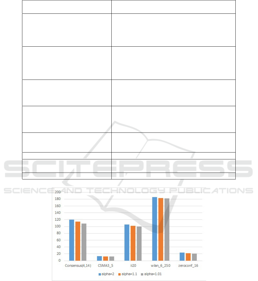
Table 1: Case Study Models.
Name Param. Number of Number of Construction and PRISM
param.s Values States transitions pre-computation time upper bound
4,8 84,096 282,592 0.7 5.36E13
Consensus 4,14 145,536 489,952 1.1 8.99E20
(n,k) 4,20 206,976 697,312 3.7 1.51E28
5,6 482,816 2,011,120 2.2 1.34E14
5,10 792,576 3,307,120 4.5 1.40E20
10,1000 3,001,911 6,787,615 97 1.54E27
Zeroconf 14,1000 4,427,159 10,009,768 162 6.37E32
(K,N) 18,1000 5,477,150 12,374,708 241 4.92E40
12, 50 3,754,386 8,489,802 127 7.35E30
16, 50 5,010,803 11,325,290 205 7.92E38
5,2000 4,419,518 9,214,380 451 1205090
Wlan 6,10 5,007,548 1,1475,748 81 1205090
(n,ttm) 6,250 5,755,628 12,976,948 163 1205090
6,1200 8,716,778 18,919,198 565 1205090
16 65,535 917,504 .3 1210869
ij 18 262,143 4,128,768 .68 6708302
(n) 20 1,048,575 18,350,080 3.5 4.82E7
22 4,194,303 80,740,352 9.1 2.13E8
3,4 1,460,287 2,396,727 6.1 718599
CSMA 3,5 12,070,354 20,214,947 28 5718599
(N,K) 4,3 8,218,017 15,384,772 15.5 8718599
leader(n) 7 2,095,783 7714385 18.5 859176
firewire 24 84,152 178,116 6.9 246000
(delay) 36 212,268 481,792 14.5 379000
MDP35 - 35 66 0.08 2
Figure 3: Running times of Algorithm 3 with three different values for the c
1
parameter.
Algorithm 3 (that also used Algorithm 2) after SCC
decomposition to compute the values of states of
each SCCs. In most cases (except the last one), our
proposed methods outperform the standard interval
iteration of PRISM. It is also the case for SCC-based
version of our improved method, compared to the
SCC-based version of sound value iteration (SCC-
SVI in Table 2). In some cases (Wlan for example)
the sound value iteration method is much faster than
our proposed methods without SCC decomposition.
The main reason is that STORM applies some
reduction techniques for these cases. However, the
SCC-based version of our method outperforms the
SCC-based sound value iteration for these cases. In
most cases, our method reduces the running time
of iterative computations to less than 50% of the
Accelerating Interval Iteration for Expected Rewards in Markov Decision Processes
47

Table 2: Running times of variant interval iteration methods.
Name Param PRISM STORM
params Values Standard Separate Improved Standard Improved SVI SCC SCC
II II II SCC-II SCC-II II SVI
4,8 48.8 45.7 20.9 37.26 11.41 25.9 43.6 24.4
Consensus 4,14 241.7 219.5 115.9 197.2 68.25 147.8 309 131
(n,k) 4,20 680.9 620 324.6 603.3 212.8 472 593 377
5,6 428.3 372 146.9 260 88.8 182 339 163
5,10 1734 1552 624 1289 439 824 1376 752
10,1000 166.4 104.3 10.5 35.4 7.97 31.1 30.5 35.9
Zeroconf 14,1000 271.6 175.1 18.56 67.1 14.55 53.1 59 63.9
(K,N) 18,1000 378 238.7 24.43 90.23 19.61 57.2 77.5 85.2
12, 50 163.9 104.6 10.9 34.4 8.7 37.4 39.8 42
16, 50 228.3 146.6 16.85 54.8 13.8 50.6 52.7 55.4
5,2000 2571 1467 680 30.1 6.1 14.7 15.2 15.5
Wlan 6,10 464.6 317.5 10.9 4.72 1.15 11.9 13.4 13.8
(n,ttm) 6,250 722.3 482.8 177.9 8.81 3.33 13.8 15.6 15.9
6,1200 2530 1545 1075 37.7 10.5 25.9 26.8 27.3
16 4.69 4.61 2.42 1.19 0.56 5.93 3.71 2.11
ij 18 48.4 46.9 16.17 10.9 4.91 42.4 22.9 13.7
(n) 20 338.9 335.4 94.8 73.5 32.9 249 142 73.1
22 2313 2412 613.3 445.2 220.4 1361 791 400
3,4 5.37 4.96 1.45 0.52 0.54 8.74 7.2 7.1
CSMA 3,5 69.6 68.9 46.8 5.86 4.17 87.4 62.4 60.3
(N,K) 4,3 44.3 44 16 4.1 3.3 67 57.7 57.5
leader(n) 7 5.99 5.34 3.79 1.77 1.6 4.73 3.52 3.31
firewire 24 1.46 1.39 0.94 0.92 0.46 2.11 1.53 1.42
(delay) 36 5.91 3.65 4.98 4.42 2.58 4.73 4.58 4.32
MDP35 - 5.14 3.78 6.2 5.16 6.22 3.19 4.53 3.22
running time of the best technique from the previous
works. More experiments are also available at
https://github.com/mohagheghivru/Asynchronous II.
For the last model, our second heuristic is unable to
satisfy the condition of lemma 1. Hence, it uses the
standard approach after several redundant iterations
for checking the condition of this lemma. It is
the main drawback of our second heuristic, which
happens for the last case study. Even in this case,
the first heuristic outperforms the standard interval
iteration and SVI methods. The computed values for
the first state of each model are reported the same in
six digits after decimal point among all approaches of
Table 2 and can be investigated through our log files
in GitHub.
Table 3 presents the total number of iterations of
each method running PRISM. It also reports the num-
ber of iterations to satisfy the condition of Lemma 3.1
(last column of Table 3). In most cases, this condi-
tion is passed after a few number of iterations. For
the last case study, this condition is not passed when
the method considers c
1
= 1.1. The results of Table
2 and Table 3 show that our first heuristic reduces the
number of iterations and the running times to half for
the Zeroconf and Wlan models.
To compare the impact of different values of the
parameter c
1
of our second heuristic (Algorithm 3),
we consider three values for it. Fig. 3 shows the
results for 5 selected models (c
1
is called α in this
figure). The results show that there is no significant
difference for different values of this parameter.
5 CONCLUSION
In this paper, two methods proposed to improve the
performance of the interval iteration method for the
expected accumulated rewards. The first method sep-
arates the iterations of the upper and lower bounds
to avoid useless updates. The second method relies
on the computations of the lower bound to select a
starting point for the upper bound. It does not need
the pre-computation for selecting the starting point of
the upper bound. A lemma is proposed to guarantee
the correctness and soundness of the interval inser-
tion method with the second heuristic. Experimental
ICSOFT 2020 - 15th International Conference on Software Technologies
48

Table 3: Number of Iterations of the Methods.
Name Param PRISM
params Values Standard Separate Improved Checking
II II II Correctness
4,8 45,924 35,172 19290 1
Consensus 4,14 160,546 116,217 52,750 1
(n,k) 4,20 317,218 231,600 106,214 1
5,6 44,982 33,978 17,287 1
5,10 154,944 102,025 44,112 1
10,1000 962 544 86 6
Zeroconf 14,1000 1,056 605 92 5
(K,N) 18,1000 1,174 642 102 5
12, 50 1,050 599 88 5
16, 50 1,106 565 96 6
5,2000 40,058 20,058 8,041 2001
Wlan 6,10 256 157 81 11
(n,ttm) 6,250 5,056 2,557 1,041 51
6,1200 24,056 12,059 4,841 1,201
16 1,560 1,119 873 1
ij 18 2,096 1,431 1,118 1
(n) 20 2,758 1,930 1,558 1
22 3,098 2,171 1,704 1
3,4 92 82 66 3
CSMA 3,5 82 72 58 3
(N,K) 4,3 164 143 107 3
leader(n) 7 96 76 56 1
firewire 24 1,588 1,379 985 10
(delay) 36 1,780 1,522 1,12 4
MDP35 - 2,895,430 2,654,592 4,160,500 Not Satisfied
results show our improved method and its SCC-based
version outperform the standard interval iteration and
the sound value iteration methods. The possibility of
using the proposed methods with sound value itera-
tion is a direction for future works.
REFERENCES
Agha, G. and Palmskog, K. (2018). A survey of statistical
model checking. ACM Transactions on Modeling and
Computer Simulation (TOMACS), 28(1):1–39.
Baier, C., de Alfaro, L., Forejt, V., and Kwiatkowska,
M. (2018). Model checking probabilistic systems.
In Handbook of Model Checking, pages 963–999.
Springer.
Baier, C. and Katoen, J.-P. (2008). Principles of model
checking. MIT press.
Baier, C., Klein, J., Leuschner, L., Parker, D., and Wun-
derlich, S. (2017). Ensuring the reliability of your
model checker: Interval iteration for markov decision
processes. In International Conference on Computer
Aided Verification, pages 160–180. Springer.
Br
´
azdil, T., Chatterjee, K., Chmelik, M., Forejt, V.,
K
ˇ
ret
´
ınsk
`
y, J., Kwiatkowska, M., Parker, D., and
Ujma, M. (2014). Verification of markov decision
processes using learning algorithms. In International
Symposium on Automated Technology for Verification
and Analysis, pages 98–114. Springer.
Chatterjee, K. and Henzinger, T. A. (2008). Value itera-
tion. In 25 Years of Model Checking, pages 107–138.
Springer.
Chen, T., Forejt, V., Kwiatkowska, M., Parker, D., and
Simaitis, A. (2013). Automatic verification of com-
petitive stochastic systems. Formal Methods in System
Design, 43(1):61–92.
Ciesinski, F., Baier, C., Gr
¨
oßer, M., and Klein, J. (2008).
Reduction techniques for model checking markov de-
cision processes. In 2008 Fifth International Con-
ference on Quantitative Evaluation of Systems, pages
45–54. IEEE.
Dai, P., Weld, D. S., Goldsmith, J., et al. (2011). Topolog-
ical value iteration algorithms. Journal of Artificial
Intelligence Research, 42:181–209.
Dehnert, C., Junges, S., Katoen, J.-P., and Volk, M. (2017).
A storm is coming: A modern probabilistic model
checker. In International Conference on Computer
Aided Verification, pages 592–600. Springer.
Forejt, V., Kwiatkowska, M., Norman, G., and Parker, D.
(2011). Automated verification techniques for prob-
Accelerating Interval Iteration for Expected Rewards in Markov Decision Processes
49

abilistic systems. In International School on Formal
Methods for the Design of Computer, Communication
and Software Systems, pages 53–113. Springer.
Haddad, S. and Monmege, B. (2014). Reachability in mdps:
Refining convergence of value iteration. In Inter-
national Workshop on Reachability Problems, pages
125–137. Springer.
Haddad, S. and Monmege, B. (2018). Interval iteration al-
gorithm for mdps and imdps. Theoretical Computer
Science, 735:111–131.
Hartmanns, A., Klauck, M., Parker, D., Quatmann, T.,
and Ruijters, E. (2019). The quantitative verification
benchmark set. In International Conference on Tools
and Algorithms for the Construction and Analysis of
Systems, pages 344–350. Springer.
Kamaleson, N. (2018). Model reduction techniques for
probabilistic verification of Markov chains. PhD the-
sis, University of Birmingham.
Katoen, J.-P. (2016). The probabilistic model check-
ing landscape. In Proceedings of the 31st Annual
ACM/IEEE Symposium on Logic in Computer Sci-
ence, pages 31–45.
Kwiatkowska, M., Norman, G., and Parker, D. (2011a).
Prism 4.0: Verification of probabilistic real-time sys-
tems. In International conference on computer aided
verification, pages 585–591. Springer.
Kwiatkowska, M., Parker, D., and Qu, H. (2011b). Incre-
mental quantitative verification for markov decision
processes. In 2011 IEEE/IFIP 41st International Con-
ference on Dependable Systems & Networks (DSN),
pages 359–370. IEEE.
McMahan, H. B., Likhachev, M., and Gordon, G. J. (2005).
Bounded real-time dynamic programming: Rtdp with
monotone upper bounds and performance guarantees.
In Proceedings of the 22nd international conference
on Machine learning, pages 569–576.
Mohagheghi, M., Karimpour, J., and Isazadeh, A. (2020).
Prioritizing methods to accelerate probabilistic model
checking of discrete-time markov models. The Com-
puter Journal, 63(1):105–122.
Puterman, M. L. (2014). Markov decision processes: dis-
crete stochastic dynamic programming. John Wiley &
Sons.
Quatmann, T. and Katoen, J.-P. (2018). Sound value itera-
tion. In International Conference on Computer Aided
Verification, pages 643–661. Springer.
Wingate, D. and Seppi, K. D. (2005). Prioritization meth-
ods for accelerating mdp solvers. Journal of Machine
Learning Research, 6(May):851–881.
ICSOFT 2020 - 15th International Conference on Software Technologies
50
