Interval-based Sound Source Mapping for Mobile Robots

Axel Rauschenberger and Bernardo Wagner

Real-Time Systems Group (RTS), Institute for Systems Engineering,

Leibniz Universit

at Hannover, Appelstraße 9A, D-30167, Hannover, Germany

Keywords:

Mobile Robotics, Sound Source Mapping, Robot Audition, Interval Analysis.

Abstract:

Auditory information can expand the knowledge of the environment of a mobile robot. Therefore, assigning

sound sources to a global map is an important task. In this paper, we ﬁrst form a relationship between the

microphone positions and auditory features extracted from the microphone signals to describe the 3D position

of multiple static sound sources. Next, we form a Constraint Satisfaction Problem (CSP), which links all

observations from different measurement positions. Classical approaches approximate these non-linear system

of equations and require a good initial guess. In contrast, in this work, we solve these equations by using

interval analysis in less computational effort. This enables the calculation being performed on the hardware of

a robot at run time. Next, we extend the approach to model uncertainties of the microphone positions and the

auditory features extracted by the microphones making the approach more robust in real applications. Last,

we demonstrate the functionality of our approach by using simulated and real data.

1 INTRODUCTION

Auditory perception has an important meaning in hu-

man life. In order to improve the human-robot inter-

action (HRI), robots also need to be capable of an-

alyzing acoustic signals. Thus, much research has

been done in the ﬁeld of Robot Audition (Argentieri

et al., 2015), (Rascon and Meza, 2017). For vari-

ous tasks it is important to estimate the direction to a

sound source, which is addresses in the ﬁeld of Sound

Source Localization (SSL). Recently, Sound Source

Mapping (SSM) became a new challenge. Here, the

goal is to assign the position of sound sources to a

map. Possible applications are localization of miss-

ing people in a disaster scenario. Overall, the result

of the mapping approach depends on:

1. Knowledge about the positions of the microphone

in a global map.

2. Auditory features extracted from the microphone

signals. Here, a major role depends on the Time

Difference of Arrival (TDoA), which describes the

time offset a signal reaches a pair of microphones.

However, the listed items cannot be determined with-

out any error, due to measurement and modeling un-

certainty.

For instance, the localization result of a mobile

robot in a global map deviates from its true position.

map

Robot Position

Robot Position:

Estimated by

Localization

Sound Source

Front-back

ambiguity

Direction towards

sound source

Estimated Direction

towards sound source

(a) Challenges of SSM. (b) Interval-based approach.

Figure 1: Challenges of SSM and our solution.

Therefore, a direction measurement to a sound

source does not correspond to the true origin (cf. Fig.

1a). Consequently, the result of combined direction

measurements from different positions (e.g. by trian-

gulation) contains an error. Another problem occurs,

if the microphone positions are incorrectly speciﬁed

according to the reference coordinate system of the

mobile robot. This systemic error inﬂuences the di-

rection measurement.

Further on, due to typical geometrical symme-

tries of the arrangement of microphones, ambigui-

ties can arise, making it impossible to distinguish be-

tween a sound source coming from the front or the

back (Front-back ambiguity). Speciﬁcally, the ﬁeld

of Binaural Audition, which uses only a single pair of

microphones (representing human ears), suffers from

this problem.

Unfortunately, in the classical approaches less at-

Rauschenberger, A. and Wagner, B.

Interval-based Sound Source Mapping for Mobile Robots.

DOI: 10.5220/0009832803350345

In Proceedings of the 17th International Conference on Informatics in Control, Automation and Robotics (ICINCO 2020), pages 335-345

ISBN: 978-989-758-442-8

335

tention is paid to address the uncertainties leading to

the mentioned problems. Therefore, in this paper,

an approach for mapping the 3D position of multiple

sound sources is developed, which is able to tackle

the aforementioned issues. Hereby, we will focus on

static sound sources.

First, we describe the physical relationship be-

tween the microphone positions and the TDoA mea-

surements (cf. Section 4). This relationship takes the

front-back ambiguity into account. However, solving

the resulting non-linear system of equations is a chal-

lenging task. Fortunately, by using methods based on

a special case of computation on sets (introducing in

Section 3.1) - so called interval analysis (Jaulin et al.,

2001) - we are able to solve the equations without

any approximation and less computational effort com-

pared to classical approaches. This is an important re-

quirement for performing the 3D SSM using the hard-

ware of a mobile robot at run time. Next, Section 5

shows our interval-based approach to solve the cor-

responding Constraint Satisfaction Problem (CSP).

As a consequence, the sound source positions are de-

scribed by boxes, depicted in Figure 1b). Afterwards,

we use another beneﬁt of the interval analysis and ex-

tend our approach to model the uncertainty of the mi-

crophone positions (cf. Section 6). Next, we propose

a novel method to estimate the TDoA from the micro-

phone signals and describe their uncertainty (cf. Sec-

tion 7). By doing this, our approach is getting more

robust in real applications. Finally, Section 8 presents

an evaluation in the simulation and in a real experi-

ment, which shows the feasibility of our approach (cf.

Section 8).

In summary, the main contributions of our

Interval-Based Sound Source Mapping (IB-SSM)

are:

• Taking front-back ambiguity into account

• Low computational effort, making it applicable

using on the hardware of a robot

• Novel method for estimating the TDoA from di-

rection measurements

• Modeling uncertainty of microphone positions

and TDoA using intervals

2 RELATED WORK

Existing approaches for SSM can be divided into two

categories. The ﬁrst category based on ray trac-

ing. These approaches assume, that the origin of a

sound source corresponds to a visible feature in a

map. Therefore, a so-called occupied grid is used,

which contains the information if grids of a geomet-

ric map are occupied or free. Next, due to SSL the

directions to the sound sources are estimated. Grids

intersecting by a ray toward this direction are assigned

with a probability representing the position of a sound

source. The main advantage of this approach is, that

with a single measurement may calculate the position

of a source. Therefore, (Kallakuri et al., 2013) uses

a 2D LiDAR to generate the occupied grid. How-

ever, the approach fails if sound sources are outside

the plane of the LiDAR (e.g. loud speaker on a table

or mounted on the ceiling). Therefore, (Even et al.,

2017) extend the approach by using a 3D LiDAR.

Disadvantages are larger cost of computation and in-

tegration of additional hardware, which cannot be ex-

tended to all existing robotic systems. Moreover, it is

assumed that sound can not pass occupied grids. As a

result, acoustical transparent materials or low walls in

front of a sound source, will be assigned with a high

probability representing a sound source.

The second category based on localization strate-

gies as Triangulation (Sasaki et al., 2010), FastSLAM

(Hu et al., 2011), Monte Carlo localization (Sasaki

et al., 2016) and Particle Filter (Evers et al., 2017). In

contrast to the ﬁrst category, measurements from vari-

ous directions need to be conducted. To overcome this

drawback (Su et al., 2016) a three layered approach is

proposed, which combines acoustic ray casting with

triangulation from (Sasaki et al., 2010). However, the

triangulation approach assumes that most cross-points

of different directions are close to the true sound po-

sition which may not be true. Further on, both cate-

gories do not address the front-back ambiguity. More-

over uncertainties for the microphone position and the

TDoA are not fully taken into account. (Sasaki et al.,

2016) models the uncertainty of a direction measure-

ment with an zero-mean Gaussian distribution. How-

ever, if the measurements are biased (i.e. they exhibit

a systematic error, due to e.g. inaccurate knowledge

about the microphone positions) this assumption will

not be true.

3 INTERVAL ANALYSIS

After introducing the interval analysis, we motivate

their usage for the task of sound source mapping.

3.1 Basics

The accuracy of a distance measurement with a fold-

ing ruler is usually ±1 mm. Here, the idea of interval

analysis arises (Jaulin et al., 2001). Instead of speci-

fying an exact value or a stochastic distribution, lower

ICINCO 2020 - 17th International Conference on Informatics in Control, Automation and Robotics

336

and upper bounds are used, deﬁned respectively by x

and x. We assume the true measurement is enclosed

in the interval [x] = [x,x]. However, no assumption is

made as to which value is most likely. By conducting

the intervals of two distance measurements A = [9,10]

and B = [2, 3] from the same reference point, we cal-

culate their interval distance as follows:

[9,10]− [2,3] = [9 − 3,10 − 2] = [6,8]. (1)

Hence, it is guaranteed that the distance is between

6 and 8. More dimensional intervals are represented

as an interval vector [x], resulting in an interval box.

Furthermore, given a measurement Y ∈ R

(e.g. the

TDoA) and a non-linear measurement function f :

→ R

the relationship to an unknown set X (e.g.

the position of the sound sources) is characterized as

follows:

X = {x ∈ R

| f(x) ∈ Y} = f

−1

(Y). (2)

The unknown set X can be calculated with a branch

and bound algorithm Set Inversion Via Interval Anal-

ysis (SIVIA) (Jaulin et al., 2001). Another approach

is to formulate f as a Constraint Satisfaction Prob-

lem (CSP) and use so-called contractors (Chabert and

Jaulin, 2009). The main idea is to start with an initial

search space containing a set of boxes. On each box

a calculation is performed and inconsistent parts are

removed, resulting in a smaller box.

3.2 Application to SSM

As we will show in Section 5, the main advantage of

using interval analysis in SSM is the simple method-

ology of solving the CSP resulting from the relation-

ship between the microphone signals (represented by

the TDoA) and their position. The solution (possible

position of sound sources) is represented by a set of

interval boxes. After conducting a subsequent mea-

surement from a different position, a new restriction is

added to the CSP. Fortunately, by using interval anal-

ysis, this process can be performed by the intersection

of the interval boxes of the previous solution. Impor-

tantly, both the microphone position and the TDoA

can also be modeled as interval boxes. By doing this,

the solution of the CSP will result in larger interval

boxes, compared to ﬁxed values for both quantities.

However, uncertainties can be modeled in a simple

manner, making it applicable for real scenarios.

First, the accuracy of the transformation between

the microphones and the reference coordinate sys-

tem at the robot is affected by the used calibration

method. This knowledge needs to be integrated to

the transformation by specifying an interval box [x].

Next, the localization accuracy of the robot within the

map depends on the used sensor and the resolution

of the map. (Langerwisch and Wagner, 2012) pro-

pose an interval-based approach for guaranteed robot

localization. In (Sliwka et al., 2011) interval meth-

ods are used in the context of robust localization of

underwater robots. Furthermore, extracting multiple

TDoA’s from the microphone signals in a noisy envi-

ronments is a challenging task. In many cases an es-

timation is given by extracting peaks from the cross-

correlation function. However, signals are sampled

at a discrete timestamp. Therefore, the uncertainty of

the TDoA highly depends on the sampling frequency.

A interval-based method to estimate the timestamps

between two sensors are proposed in (Voges and Wag-

ner, 2018).

4 PROBLEM DEFINITION AND

NOTATION

Let us assume, various sound sources s ∈ {1,...,n

}

are emitting acoustical signals with the velocity of

sound c in the current environment. n

is the total

number of sources, which is unknown in advance.

Their positions are characterized by x

∈ R

. Fur-

ther, a mobile robot perceives these acoustic signals

using a microphone array, equipped with n

micro-

phones. We model the relationship between micro-

phone pairs. Therefore, we denote the ﬁrst and second

position of a microphone pair i ∈ {1,..., n

} as x

(n)

i,1

and x

(n)

i,2

∈ R

. n

is the total number of used micro-

phone pairs. Due to the movement of the robot, the

positions of the microphones are changing. There-

fore, the superscript n ∈ {1,.., n

} denotes the index

of location and n

is the total number of locations.

Moreover, the time a signal arrives at the ﬁrst and

the second microphone results in a time difference -

so-called Time Difference of Arrival (TDoA) - which

we denote as

(s)

∆t

(n)

. The superscript s indicates the

TDoA resulting from source s. Further, the TDoA

depends on the position of microphone pair i at loca-

tion index n. Finally, we form a relationship between

the position of a microphone pair and the TDoA mea-

sured for a single source s as followed:

||x

(n)

i,1

− x

− ||x

(n)

i,2

− x

(s)

∆t

(n)

· c. (3)

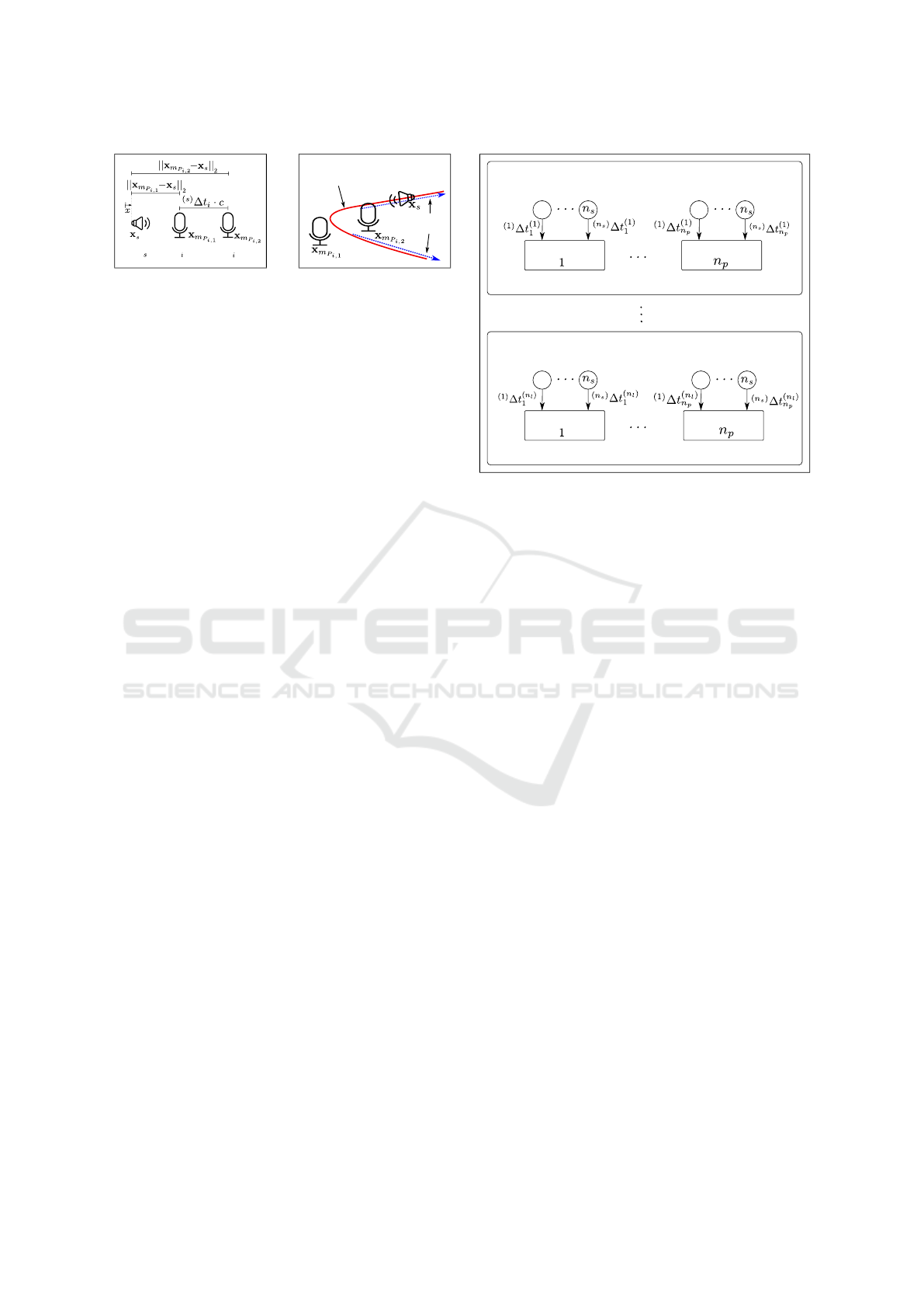
For an easier understanding we show the relation-

ship in Fig. 2a dropping the superscript (n). It can

be noted that, the left-hand side of Equation (3) con-

tains the geometrical properties of the microphone

conﬁguration, whereas the right-hand side includes

the measurements of the microphone pair in form of

Interval-based Sound Source Mapping for Mobile Robots

337

First microphone

from pair

Second microphone

from pair

Sound

Source

(a) Relationship between the position

of a microphone pair and the TDoA

given in Equation (3).

Possible position of

sound source s

Front-back

ambiguity

(b) The position of a sound source is

located on a hyperbolic curve (red) for

a given TDoA.

Figure 2: Relationship between microphone signals and

their position.

the TDoA. As indicated in Figure 2b the solution of

Equation (3) for a ﬁxed TDoA is located on a hyper-

bolic curve. By making the assumption that a sound

source is far away (far ﬁeld assumption), two feasi-

ble directions towards the sound sources can be occur,

which represents the front-back ambiguity (cf. Fig.

2b). In contrast to presented methods in Section 2, we

do not restrict our approach to these directions. In-

stead we use the information of the hyperbolic func-

tion to infer the sound position.

Next, Equation (3) only describes the relation-

ship between a single microphone pair for one sound

source at one measurement position. However, each

microphone pair perceives various sound sources at

different measurement positions (cf. Fig. 3). Thus,

the total number n

of equations is stated as follows:

= n

· n

. (4)

Therefore, we integrate all equations into a mathemat-

ical system, which needs to be solved. Due to the high

non-linearity and restriction between all equations,

this is a challenging task. Classical approaches lin-

earize each equation through a second order Taylor-

series expansion (Foy, 1976), but suffer from inten-

sive computation and require a good initial guess. In

contrast to these approaches an interval-based method

is proposed in (Reynet et al., 2009). Though, Equa-

tion (3) is solved in a different context of localizing

the origin of an electromagnetic wave emitting source

by using three static receivers for a known TDoA. We

found that this approach can be applied to our prob-

lem. Therefore, we deﬁne the methodology in the

next Section.

5 RESULTING CONSTRAINT

SATISFACTION PROBLEM

In this Section we calculate a set of interval boxes

which includes all sound sources positions of the en-

vironment.

Sound Sources

Microphone pair

Measurement position 1

Sound Sources

Microphone pair

Measurement position n

Sound Sources

Microphone pair

Sound Sources

Microphone pair

Figure 3: Equation (3) needs to be fulﬁlled for all micro-

phone pairs, all sound sources at all measurement positions.

Therefore, we formulate Equation (3) as a CSP as

follows:

H :











Variables: x

Constants: x

(n)

i,1

(n)

i,2

(s)

∆t

(n)

Contraints:

1. ||x

(n)

i,1

− x||

− ||x

(n)

i,2

− x||

(s)

∆t

(n)

· c

Domains: [x

],[x

(n)

i,1

],[x

(n)

i,2

],[

(s)

∆t

(n)

],[c]

Depending on the assignment of the domain, we are

able to model uncertainties. Furthermore, if the do-

main of the values are selected in a proper way, it can

be guaranteed that the true solution is included. How-

ever, specifying these bounds is a challenging task.

The bounds of the velocity of sounds c depend on the

range of temperature in the environment. In this work,

we set the bounds for the microphone positions as ex-

plained in Section 6. In Section 7, we show the pro-

cess of estimating the bounds for the TDoA from the

microphone signals.

To solve the CSP H we use the branch and bound

algorithm Set Inversion Via Interval Analysis (SIVIA)

(Jaulin et al., 2001) and a forward-backward contrac-

tor (Chabert and Jaulin, 2009), which we denote with

(s)

(n)

. The main idea is that we start with an ini-

tial box [x] containing the full dimension of the con-

sidered environment. Afterwards, we perform calcu-

lations on [x] using the contractor

(s)

(n)

, which re-

moves inconsistent parts of [x].

The formulated CSP describes the position of a

single sound source s according to one microphone

ICINCO 2020 - 17th International Conference on Informatics in Control, Automation and Robotics

338

pair i at the measurement position n. However, the

position of s needs to be included in all equations cor-

responding to the other microphone pairs. Therefore,

in the ﬁrst step we need to identify all equations at

the position n describing the relationship to the sound

source s (cf. Section 7). Afterward, due to the ben-

eﬁts of interval analysis, we form a single contractor

for all of these microphone pairs, by intersection of

the corresponding contractors:

Contractor Source s:

(s)

(n)

i=1

(s)

(n)

. (5)

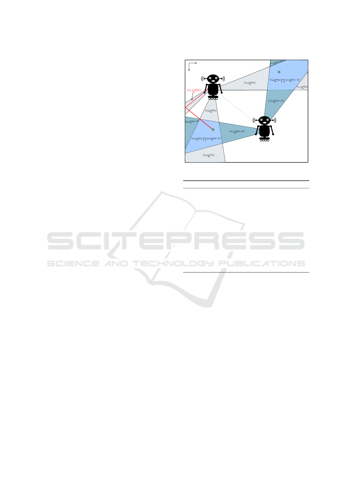
To visualize the applied methodology, we illus-

trate the mapping of a sound source in the schematic

draw in Fig. 4. The signals of two sources s

and

are perceived by a mobile robot at position n and

n + 1. Additionally, at position n a reﬂection s

from

sound source s

occurs. At each position and for each

sound source a contractor

(s)

(n)

is calculated. Using

each contractor separately on [x] results in ﬁve areas,

which are not linked. To solve this, we ﬁrst combine

all contractors corresponding to the same position, by

calculating the union as follows:

Contractor at Position n: C

(n)

[

s=1

(s)

(n)

. (6)

Last, intersecting both contractor at position n and

n + 1, results in the ﬁnal contractor, which is used

to calculate the solution after collecting all measure-

ments.

Final Contractor: C =

n=1

(n)

. (7)

It is important to note, that these approach enable

to handle wrong direction measurements caused by

reﬂections. As, calculating the intersection results in

an empty set for areas corresponding to the reﬂec-

tions.

In summary, our Interval-Based Sound Source

Mapping (IB-SSM) is shown in Algorithm 1. After

conducting a measurement at position n (cf. line 4)

the intervals for the microphone positions (cf. line 5)

and for the TDoA (cf. line 6) are estimated. Next, the

contractor from Equation (6) is calculated (cf. line 7).

Afterward, the previous solution (or the initial domain

if ﬁrst measurement is conducted) is reduced by using

the contractor and SIVIA (cf. line 8). In contrast to

building the ﬁnal contractor C from Equation (7) after

conducting all measurements, the proposed algorithm

beneﬁts from new information directly after conduct-

ing a measurement. This enables optimal positions to

be calculated at run-time making it feasible to result

in a more accurate solution.

Robot at

Position n

Robot at

Position n+1

map

Sound

Source s

Sound

Source s

Trajectory

from Position

n to n+1

Reﬂection of s

Figure 4: Simpliﬁed representation of the contracted areas.

Algorithm 1: Pseudo-Code: IB-SSM.

Input: Initial Domain: [x], Number of Positions: n

Output: Contracted Domain [x

]

1: for n = 1 to n

2: p ← getNextMeasurementPosition(n)

3: driveToPosition(p)

4: z ← takeMeasurement(p)

5: [m] ← calcIntMicPos(p)  cf. Section 6

6: [t] ← calcIntTDoA(z)  cf. Section 7

7: C ← buildContractor([m],[t])  cf. Section 5

8: [x

] ← contractBoxes(C ,[x])  cf. Section 5

9: [x] ← [x

]

10: end for

6 INTERVAL-BASED

MICROPHONE POSITION

In order to solve the CSP from Section 5 the micro-

phone positions need to be known. In our proposed

approach we model the following aspects:

1. Error of microphone position in the coordinate

system of the mobile platform

2. Localization error of the mobile platform

First, we measure the translation t

∈ R

between a

ﬁxed coordinate system on the platform to the center

of a microphone membrane m

. This translation is the

outcome of a calibration process. Here, we do not as-

sume any directivity of the microphones, therefore no

orientation is modeled. Last, depending on our cal-

ibration method we extend t

in all dimension with

an uncertainty t

∈ R

and model the result as an in-

terval box [t

− t

+ t

]. Great attention has to

be given to these bounds. However, even for a poor

Interval-based Sound Source Mapping for Mobile Robots

339

calibration it can be guaranteed, that the true position

of the sound sources are included in the result of our

SSM approach, if proper bounds are selected.

Second, the transformation from the coordinate sys-

tem of the mobile platform to a global map is given

as:

(map)

= R

map

rob

(rob)

map

rob

. (8)

map

rob

denotes the translation from the mobile coordi-

nate system to the map coordinate system.

map

rob

∈ SO(3) models the rotation. Because the

movement of the mobile platform is restricted to the

XY-plane, a rotation only occurs around the z-axis.

Thus, R

map

rob

can be described as follows:

map

rob





cos(α) −sin(α) 0

sin(α) cos(α) 0

0 0 1





. (9)

Depending on the used localization algorithm the

translation t

map

rob

is extended with an uncertainty e.g.

described above. Here, special consideration needs to

be paid to the resolution of the used map. Next, the

bounds for the angle α need to be speciﬁed.

7 INTERVAL-BASED TIME

DIFFERENCE OF ARRIVAL

The time differences of microphone pairs are required

in order to solve the CSP in Section 5. Fig. 3 shows

that a single microphone pairs needs to distinguish

TDoA’s corresponding to n

different sources. With-

out any additional knowledge about the characteris-

tics of the signals it is a challenging task. Follow-

ing approaches can be used to address the problem of

ﬁnding intervals for the TDoA:

1. Interval-based approach using the raw micro-

phone signals

2. Direction measurements through state-of-the-art

methods from the ﬁeld of Sound Source Localiza-

tion (SSL) combined with tracking methods

It should be noted, that the ﬁrst approach is the best

choice in order to calculate guaranteed bounds for the

time differences.

However, addressing this problem without any

knowledge about the characteristics (e.g frequency

range of signals) is hard to handle. We do not as-

sume about these characteristics, resulting in a higher

range of applications. Due to the robustness against

noise in real applications, by using tracking methods

with existing SSL, we focus on the second approach.

By doing this, existing SSL systems can be easily

extended to perform SSM. The most promising ap-

proaches for SSL are subspace methods derived from

Input:

Microphone

Signals

SSL

(e.g. SRP-PHAT,

MUSIC)

M3K method

Tracked

Directions

Collect

Directions

Measurement

Duration:

Collected

Directions

Cluster

Directions

K-mean

Clustering

Clustered

Directions

Calculate

Angle Bounds

for each cluster

Add System

bounds

SSL-Resolution

Calculate

Time Diﬀerence

Append

Sampling Error

Extended Cone

Segments

Cone

Segments

Direction projected

on unit sphere

Cluster

Output:

Time Diﬀerence

Interval for each

Cluster

Figure 5: Pipeline for calculating the time difference inter-

vals.

MUSIC (Schmidt, 1986) e.g. GEVD-MUSIC (Naka-

mura et al., 2009) and beamforming-based methods

e.g. SRP-PHAT (Do et al., 2007). A comprehen-

sive review of existing SSL approaches is given in

(Rascon and Meza, 2017). These approaches esti-

mate the Direction of Arrival (DoA) to a sound source

s represented by azimuth (horizontal angle) θ

and

(vertical angle). The angle conventions are given

in Fig. 6. However, the direct result of these algo-

rithms without any post-processing is not practical in

real experiments. For this reason, we use a modiﬁed

3D Kalman (M3K) method proposed in (Grondin and

Michaud, 2019). The direction of the SSL is classiﬁed

as three possible states: diffuse noise, emitting from

a new sound source, or emitting from a tracked sound

source. For the following and our experiments in Sec-

tion 8.2 we only use directions from tracked sources.

Furthermore, using SSL algorithms in practice,

the system is getting more robust against noise by col-

lecting various measurements in a speciﬁc duration of

time t

. We assume all sound sources s being active

for at least 20 percent of this time. A set of direc-

tions is computed after the measurement (see Fig. 5).

Hence, we cluster these directions characterized by

projecting the directions on a unit sphere - by the k-

mean algorithm.

We calculate for each cluster the bounds for the

angles [θ

,θ

] and [φ

,φ

] by selecting the minimal

and maximal values. Attention should be paid to

the angle resolution of the used SSL algorithm and

it needs to be appended at the intervals for θ

and φ

In order to prevent collisions with the sound

sources and to eliminate disturbances by the

robot/sensor setup itself we restrict all sound sources

s being located at least with the minimal distance r

the microphone array. The maximal distance r

results

from the structure of the room. Altogether, the posi-

tion of each sound source is assumed being located in-

ICINCO 2020 - 17th International Conference on Informatics in Control, Automation and Robotics

340

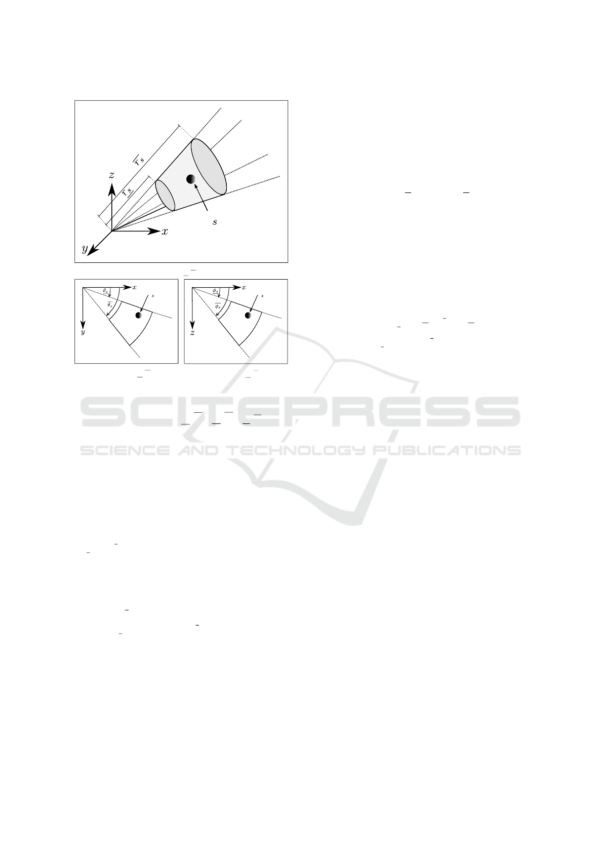
Sound Source

(a) 3D view: Bounds [r

] for radius r.

Sound Source

(b) XY-Plane: Bounds [θ

,θ

] for az-

imuth θ.

Sound Source

,φ

] for ele-

vation φ.

Figure 6: Segment cone.

side a cone segment con

([φ

,φ

],[θ

,θ

],[r

]) ∈ R

visualized in Figure 6a.

It is quite important to underline that, due to front-

back confusion, the sound sources may not be in-

cluded in this area. As a conclusion, the area of

the cone segment can not directly be used to infer

the sound source positions. Instead, the time differ-

ences resulting from points inside the segment cone

∈ con

and the position of a pair of microphones

can be used to solve this problem by computing the

CSP in Section 5. As a result we obtain an interval

[

(s)

(n)

(s)

(n)

] which describes the minimal and max-

imal time difference for each microphone pair i ac-

cording to the cone segment for a single sound source

s. There, the calculation is given as:

(s)

(n)

(||x

(n)

i,1

− x

− ||x

(n)

i,2

− x

(s)

(n)

= min

(s)

(n)

(s)

(n)

= max

(s)

(n)

(10)

However, even this interval may not include the true

TDoA in a real application due to the discrete sam-

pling of the microphone signals. For instance, a signal

reaches at t

= 0.95 ms the ﬁrst and at t

= 0.3 ms the

second microphone. By selecting the sampling time

= 0.2 ms of the acoustic signal, both values can not

be perceived accurately. Instead, we build an interval

as follows:

[a] = [t

−t

] = [0.75, 1.15]

[b] = [t

−t

] = [0.1, 0.5].

As a result the time difference is calculated as follows:

[a] − [b] =

−t

− 2 ·

−t

+ 2 ·

] =

[0.25,1.05].

Therefore, it is guaranteed, that the time difference

is between 0.25 ms and 1.05 ms. To enable a com-

parison to real applications, the sampling frequency

usually is in the range of 8000 to 96000 Hz resulting

in a sampling time of 0.01 ms to 0.125 ms.

We use these description of modeling uncertain-

ties to extend the interval of time differences as fol-

lows:

(s)

(n)

= [

(s)

(n)

−

(s)

(n)

] =

[

(s)

(n)

− ∆t

(s)

(n)

+ ∆t

Here, ∆t

describes the extension of the interval,

which we denote as TDoA sampling extension.

8 SIMULATION AND

EXPERIMENTAL RESULTS

We validated our approach using simulated and real

data. Various simulations were conducted showing

the capabilities of our approach. First we showed

that the solution of our approach contains in all cases

the true sound source position if we are using ground

truth data. Next, we conducted various experiments

showing the inﬂuence of different parameters to the

solution of our approach. Furthermore we showed the

feasibility of our approach to handle systematic errors

(inaccurate robot localization). Finally, we performed

a experiment showing the feasibility of our approach

in a real environment.

8.1 Simulation Results

We evaluated our approach using simulated data using

Gazebo (Koenig and Howard, 2004) and implemented

our interval-based Sound Source Mapping (IB-SSM)

using the IBEX library (Ninin, 2015). In order to ne-

glect the inﬂuence on the used SSL approach we used

simulated direction measurements. These directions

are used to calculate the TDoA in Equation (10). For

all experiments in this Section we used a ﬁxed con-

ﬁguration of 8 microphones leading to n





= 28

microphone pairs (cf. Fig. 1b).

Interval-based Sound Source Mapping for Mobile Robots

341

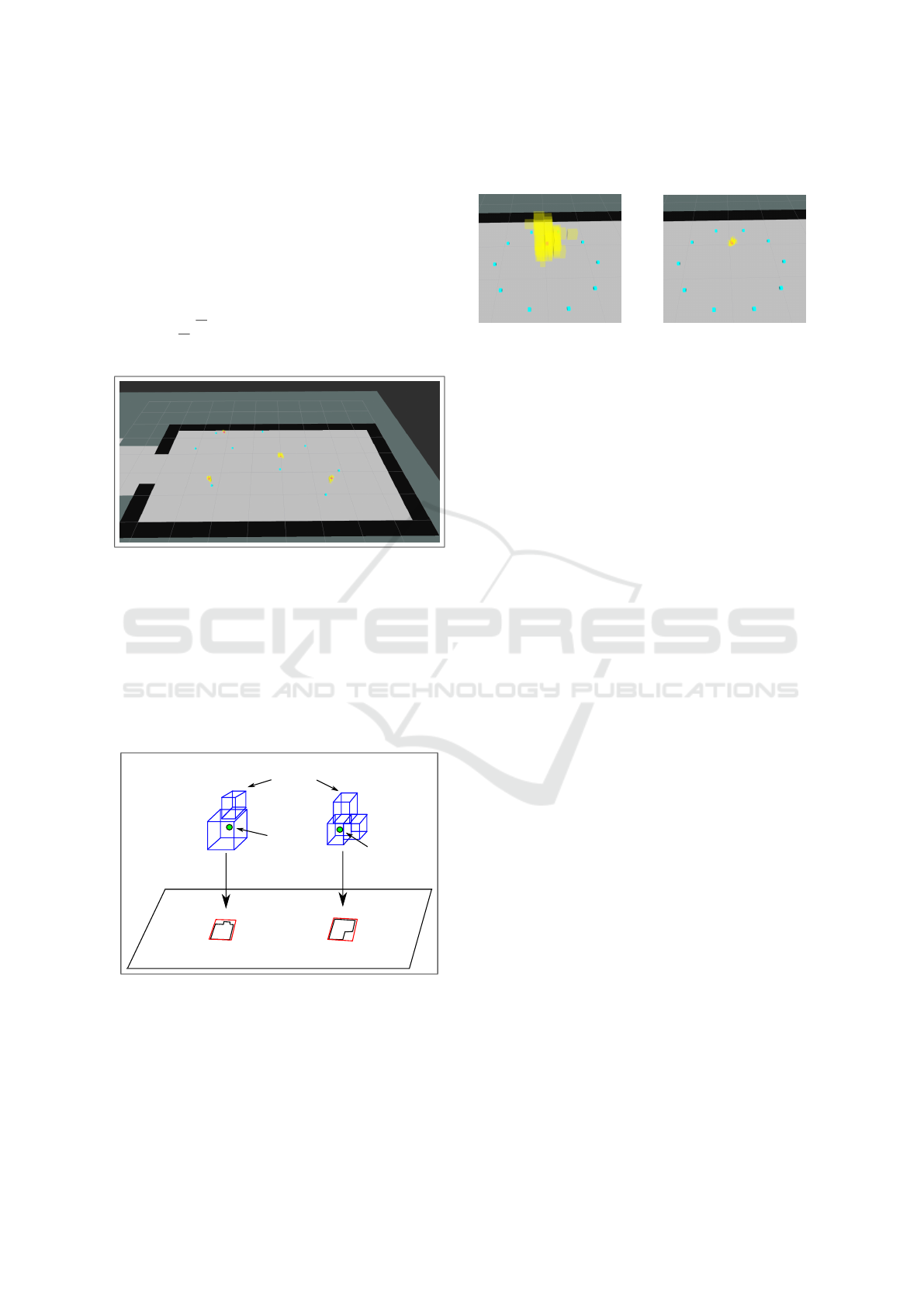
In the ﬁrst experiment we tested the feasibility of

our approach using ground truth data. In 1000 trials

we placed randomly 1-10 sound sources in the virtual

environment (7.6 m ×5.5 m ×2 m) and conducted

measurements at 1-30 positions. Fig. 7 shows a single

scenario.

In order to calculate the cone segment in Equa-

tion (10) we set the minimal and maximal distance

between the measurement and the sound sources po-

sitions to [r

] = [0.5 m,9.6 m] based on the dimen-

sion of the environment and the microphone conﬁgu-

ration.

Figure 7: Measurement positions (blue), sound source po-

sitions (red), estimated interval boxes (yellow).

For all tests, we noticed that our method includes

all true sound positions.

In the second experiment, we evaluated the inﬂu-

ence of different parameters on the accuracy of our

approach. After solving the CSP from Section 5 we

obtain a list of boxes. However, we do not get any as-

signment between these boxes and the sound sources.

2D plane

Projected bounds

for s

Projected bounds

for s

Sound source

Estimation of sound position

using Interval boxes

Figure 8: Approach to extract corresponding boxes to a

sound source.

In order to calculate the accuracy of our approach

we cluster these boxes. First, we project the boxes to

the XY plane and perform morphological methods to

obtain neighboring areas. Next, we calculate bounds

which contain these separate areas. In the last step,

we add up the volume of all interval boxes which cor-

responding to these bounds.

(a) Accuracy ε = 0.3. (b) Accuracy ε = 0.05.

Figure 9: Inﬂuence on the accuracy of SIVIA. Measurement

positions (blue), sound source positions (red), solution of

IB-SSM (yellow).

We focused on the following parameters:

• n

: Number of measurement positions

• d : Distance between measurement position and

sound source

• ε : Accuracy of the brand and bound algorithm

SIVIA used for solving the CSP

• ∆t

: TDoA sampling extension

To simplify the evaluation in this work, we did not fo-

cus on different microphone conﬁgurations. For the

following experiment we conducted measurements

located on a circle and placed a single sound source

in the center at a height of 1 m. We varied the to-

tal amount of measurement positions n

from 1 to 20,

the radius of the circle d from 0.5 m to 2 m and the

accuracy ε of SIVIA between 0.1 and 0.3. In simple

terms, ε speciﬁes the dimension of the interval boxes

showing in Fig. 9. The calculated TDoA from Section

7 needs to be extended by the TDoA sampling exten-

sion ∆t

in Equation (11). We selected a minimal sam-

pling frequency f

of 8000 Hz resulting in a sampling

time t

of 0.125 ms. Therefore, we selected the TDoA

sampling extension ∆t

between 0 ms and 2/ f

= 0.25

ms. For all combination of these aforementioned pa-

rameters we calculated the total volume of the inter-

val boxes and the calculation time of our IB-SSM al-

gorithm using the ﬁnal contractor from Equation (7).

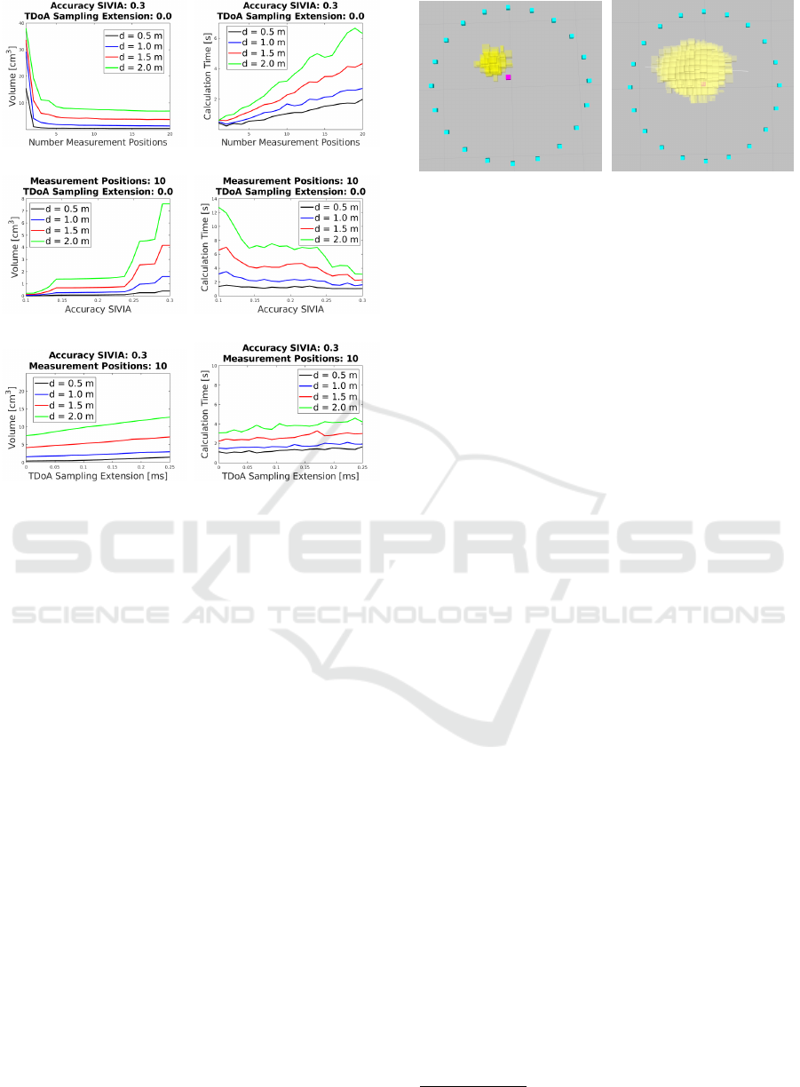
The results are visualized in Fig. 10.

Fig. 10a and Fig. 10b show that more measure-

ment positions lead to a more accurate solution but

the calculation time increases. However, at a certain

point, only a small improvement is possible. It can be

seen that the distance between the robot and the sound

source is important. Measurements at two positions

with a distance of 0.5 m to the sound source are lead-

ing to a more accurate solution than 20 measurements

point from a distance of 1 m. As a result, selecting op-

timal measurement positions should be evaluated in

following works. Furthermore, Fig. 10c and Fig. 10d

ICINCO 2020 - 17th International Conference on Informatics in Control, Automation and Robotics

342

(a) (b)

(e) (f)

Figure 10: Dependency of the total volume of all interval

boxes and the measurement time due to the number of mea-

surements (a) + (b), the accuracy of SIVIA (c) + (d) and the

TDoA sampling extension (e) + (f).

show the inﬂuence on the volume and the calculation

time caused by the accuracy ε. For d = 2 m a smaller

ε (higher accuracy) results in a large improvement.

The volume decreases from 7.6 to 0.2 cm

. However,

the calculation time rises up from 3.1 to 12.7 seconds.

For d = 0.5 m the improvement is not large (from 0.4

to 0.0129 cm

) and the calculation time is nearly con-

stant (from 1.06 to 1.36 seconds). As a result, a trade-

off between the accuracy and the calculation time has

to be made. Last, Fig. 10e and Fig. 10f show the in-

ﬂuence on the volume and the calculation time caused

by the TDoA sampling offset ∆t

. For a sampling fre-

quency of 8000 Hz (∆t

= 0.25 ms) and a sampling

frequency of 96000 Hz (∆t

= 0.02 ms) the volume

of the interval boxes for d = 2 m differs between 7.9

and 12.7 cm

for d = 0.5 m between 1.49 cm

and 0.40 cm

. The calculation time is slowly rising

for increasing ∆t

In the last experiment, we modeled a systematic

localization error of 0.15 m in both x and y (plane

of the ground). We selected n

= 20, d = 1 m, ε =

0.3 and ∆t

= 0 ms. Furthermore, we extended the

transformation t

map

rob

between the measurement posi-

tion (robot) and the global map from Equation (8) in

(a) Without error modeling. (b) With error modeling.

Figure 11: Systematic error of the localization result. Mea-

surement positions (blue), sound source positions (cyan),

estimated interval boxes (yellow).

both dimension with a bound of 0.15 m. In the ﬁrst

test, we did not consider the localization error from

Section 6 in our approach. Following, in the second

test we took this error into account. It can be seen

in Fig. 11a, that without consideration of systematic

errors the true solution is not within the calculated in-

terval boxes. In contrast, by considering uncertainties

with intervals the true solution is included but the vol-

ume is 12 times larger, see Fig. 11b.

8.2 Experimental Results

In this experiment, we provided a proof of concept,

showing our approach is applicable in a real environ-

ment. We restricted our evaluation on one single ac-

tive sound source. For this purpose, we used loud

speaker of a phone emitting speech.

The experiment was conducted in a room (11.7 m

x 6 m) using a KUKA youBot equipped with a mi-

crophone array (IntRoLab 8SoundUSB) with 8 mi-

crophones sampled with 44100 Hz as shown in Fig.

12. We used the ODAS

framework (Open em-

beddeD Audition System) for estimating the sound

source directions. The SRP-PHAT-HSDA algorithm

with a M3K method is applied (Grondin and Michaud,

2019). We used gmapping, an openSLAM imple-

mentation (Grisetti et al., 2007) and amcl (Adaptive

Monte-Carlo localization) to localize the robot within

the environment. Both are packages within the Robot

Operating System (ROS) (Quigley et al., 2009). All

algorithm were executed on the hardware of the robot.

First, we restricted our domain as shown in Fig. 13

and assumed a localization error of 0.03 m. We col-

lected for a duration of 5 seconds the tracked direction

estimations using the M3K method. After collection

all measurements at a position we calculated the so-

lution of the sound source mapping. The results are

shown in Fig. 13.

http://odas.io

Interval-based Sound Source Mapping for Mobile Robots

343

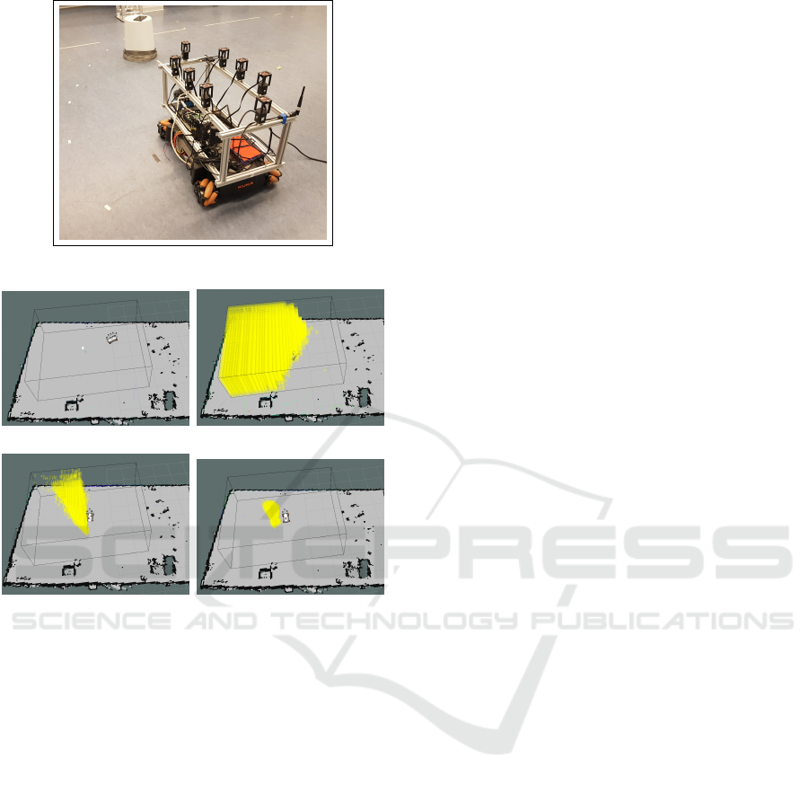
Figure 12: Experimental equipment.

(a) Start. (b) After measurement 1.

Figure 13: Results of IB-SSM (potential sound sources as

boxes in yellow) in a real environment. One static sound

source is active (white).

At the ﬁrst position, we selected a large ε to reduce

calculation time. Next, we applied the results from

the evaluation in Section 8.1 and navigated toward the

area of the sound sources and we reduced ε. After

conducting the third measurement we could show that

the true position is included in our calculated solution.

9 CONCLUSION AND FUTURE

WORK

We presented a new approach for estimating the 3D

position of multiple static sound sources in a map by

using interval methods in an efﬁcient manner. As a

result a calculation on a robot at run time is feasible.

We extended our Interval-Based Sound Source Map-

ping (IB-SSM) in order to model uncertainties due to

inaccurate knowledge about the microphone positions

within the map and the auditory signals extracted by

the microphones. Furthermore, we developed an ap-

proach to estimate the TDoA from direction measure-

ments. Our evaluation showed that our approach is

feasible to correctly estimate the positions of emitting

sound sources. In future work we plane to develop

a strategy to selected optimal measurement points in

the environment.

REFERENCES

Argentieri, S., Danes, P., and Soueres, P. (2015). A survey

on sound source localization in robotics: From binau-

ral to array processing methods. Computer Speech &

Language, 34(1):87–112.

Chabert, G. and Jaulin, L. (2009). Contractor programming.

Artiﬁcial Intelligence, 173:1079–1100.

Do, H., Silverman, H. F., and Yu, Y. (2007). A real-time srp-

phat source location implementation using stochas-

tic region contraction (src) on a large-aperture micro-

phone array. In Acoustics, Speech and Signal Process-

ing, 2007. ICASSP 2007. IEEE International Confer-

ence on, volume 1, pages I–121. IEEE.

Even, J., Furrer, J., Morales, Y., Ishi, C. T., and Hagita, N.

(2017). Probabilistic 3-d mapping of sound-emitting

structures based on acoustic ray casting. IEEE Trans-

actions on Robotics, 33(2):333–345.

Evers, C., Dorfan, Y., Gannot, S., and Naylor, P. A. (2017).

Source tracking using moving microphone arrays for

robot audition. In Acoustics, Speech and Signal Pro-

cessing (ICASSP), 2017 IEEE International Confer-

ence on, pages 6145–6149. IEEE.

Foy, W. H. (1976). Position-location solutions by taylor-

series estimation. IEEE Transactions on Aerospace

and Electronic Systems, (2):187–194.

Grisetti, G., Stachniss, C., and Burgard, W. (2007).

Improved techniques for grid mapping with rao-

blackwellized particle ﬁlters. IEEE transactions on

Robotics, 23(1):34–46.

Grondin, F. and Michaud, F. (2019). Lightweight and opti-

mized sound source localization and tracking methods

for open and closed microphone array conﬁgurations.

Robotics and Autonomous Systems, 113:63–80.

Hu, J.-S., Chan, C.-Y., Wang, C.-K., Lee, M.-T., and Kuo,

C.-Y. (2011). Simultaneous localization of a mobile

robot and multiple sound sources using a microphone

array. Advanced Robotics, 25(1-2):135–152.

Jaulin, L., Kieffer, M., Didrit, O., and Walter, E. (2001).

Interval analysis. In Applied interval analysis, pages

11–43. Springer.

Kallakuri, N., Even, J., Morales, Y., Ishi, C., and Hagita,

N. (2013). Probabilistic approach for building audi-

tory maps with a mobile microphone array. In 2013

IEEE International Conference on Robotics and Au-

tomation, pages 2270–2275. IEEE.

Koenig, N. and Howard, A. (2004). Design and use

paradigms for gazebo, an open-source multi-robot

simulator. In 2004 IEEE/RSJ International Confer-

ence on Intelligent Robots and Systems (IROS)(IEEE

ICINCO 2020 - 17th International Conference on Informatics in Control, Automation and Robotics

344

Cat. No. 04CH37566), volume 3, pages 2149–2154.

IEEE.

Langerwisch, M. and Wagner, B. (2012). Guaranteed mo-

bile robot tracking using robust interval constraint

propagation. In International Conference on In-

telligent Robotics and Applications, pages 354–365.

Springer.

Nakamura, K., Nakadai, K., Asano, F., Hasegawa, Y., and

Tsujino, H. (2009). Intelligent sound source localiza-

tion for dynamic environments. In 2009 IEEE/RSJ In-

ternational Conference on Intelligent Robots and Sys-

tems, pages 664–669. IEEE.

Ninin, J. (2015). Global optimization based on contractor

programming: An overview of the ibex library. In

International Conference on Mathematical Aspects of

Computer and Information Sciences, pages 555–559.

Springer.

Quigley, M., Conley, K., Gerkey, B., Faust, J., Foote, T.,

Leibs, J., Wheeler, R., and Ng, A. Y. (2009). Ros: an

open-source robot operating system. In ICRA work-

shop on open source software, volume 3, page 5.

Kobe, Japan.

Rascon, C. and Meza, I. (2017). Localization of sound

sources in robotics: A review. Robotics and Au-

tonomous Systems, 96:184–210.

Reynet, O., Jaulin, L., and Chabert, G. (2009). Robust tdoa

passive location using interval analysis and contractor

programming. In 2009 International Radar Confer-

ence” Surveillance for a Safer World”(RADAR 2009),

pages 1–6. IEEE.

Sasaki , Y., Ryo, T., and Takemura, H. (2016). Probabilistic

3d sound sources mapping using moving microphone

array. In Intelligent Robots and Systems (IROS), 2016

IEEE/RSJ International Conference on. IEEE.

Sasaki, Y., Thompson, S., Kaneyoshi, M., and Kagami,

S. (2010). Map-generation and identiﬁcation of

multiple sound sources from robot in motion. In

2010 IEEE/RSJ International Conference on Intelli-

gent Robots and Systems, pages 437–443. IEEE.

Schmidt, R. (1986). Multiple emitter location and signal

parameter estimation. IEEE transactions on antennas

and propagation, (3):276–280.

Sliwka, J., Le Bars, F., Reynet, O., and Jaulin, L. (2011).

Using interval methods in the context of robust local-

ization of underwater robots. In 2011 Annual Meeting

of the North American Fuzzy Information Processing

Society, pages 1–6. IEEE.

Su, D., Nakamura, K., Nakadai, K., and Valls Miro, J.

(2016). Robust sound source mapping using three-

layered selective audio rays for mobile robots. In In-

telligent Robots and Systems (IROS), 2016 IEEE/RSJ

International Conference on. IEEE.

Voges, R. and Wagner, B. (2018). Timestamp offset cal-

ibration for an imu-camera system under interval un-

certainty. In 2018 IEEE/RSJ International Conference

on Intelligent Robots and Systems (IROS), pages 377–

384. IEEE.

Interval-based Sound Source Mapping for Mobile Robots

345