Bee-route: A Bee Algorithm for the Multi-objective Vehicle Routing

Problem

Jamila Sassi

, Ines Alaya

and Moncef Tagina

COSMOS-ENSI, National School of Computer Sciences, University of Manouba 2010, Tunisia

Keywords:

Combinatorial Multi-objective Optimization, Artiﬁcial Bee Colony Algorithm (ABC), Multi-objective

Vehicle Routing Problem with Time Window (VRPTW).

Abstract:

The vehicle routing problem has attracted a lot of interest during many decades because of its wide range

of applications in real life problems. This paper aims to test the efﬁciency and capability of bee colony

optimization for this kind of problem. We present a Bee-route algorithm: a multi-objective artiﬁcial Bee

Colony algorithm for the Vehicle Routing Problem with Time Windows. We have performed our experiments

on well known benchmarks in the literature to compare our proposed algorithm results with other state-of-the-

art algorithms.

1 INTRODUCTION

The vehicle routing problem (VRP) is a part of a

large application domain. It could be applied to var-

ious ﬁelds such as transportation, network connec-

tion, health management techniques, recycling meth-

ods, etc. The VRP aims at ﬁnding an optimal set of

routes for a number of vehicles, initially located at a

depot, to serve a given set of customers. Each vehi-

cle leaving the depot returns to the initial depart af-

ter having completed its tour in a certain time slot.

The cumulative demand of customers visited by a ve-

hicle must not exceed its capacity. We introduce in

this article a multi-objective artiﬁcial Bee Colony al-

gorithm for Vehicle Routing Problem with Time Win-

dows (VRPTW) called Bee-route algorithm. In the

multi-objective VRPTW, we consider two objectives

to be optimized: the ﬁrst is to minimize the number of

vehicles used to deliver the demand of customers and

the second objective is to minimize the total distance

of the routes.

Approaches proposed in recent decades have been

characterized by prioritizing customers, and for time

optimization, reaching a reasonable time frames. The

problem of Vehicle Routing Problems with Time

Windows (VRPTW) constitutes a generalization of

the VRP in which each customer has a window of

time within this time the customer must be served.

https://orcid.org/0000-0002-9857-6467

https://orcid.org/0000-0002-7037-3326

The VRPTW aims to determine optimal routes for a

number of vehicles when serving a set of customers

within predeﬁned time intervals (the time windows).

The main formulation of the VRPTW was proposed in

1987 by (Solomon, 1987) where the time constraints

must be respected by each vehicle. In fact, it has been

shown that the classic VRP problem is NP-hard, and

this result could be extended to the VRPTW. While

it is quite possible to determine an optimal solution

for small instances, it quickly becomes unfeasible for

medium or large instances.

Given the complexity of the VRPTW, many res-

olution methods have been developed. In (Lim and

Zhang, 2007), proposed a two-stage algorithm for

the VRPTW. The authors extended the VRPTW algo-

rithm for m-VRPTW. Vehicle routing problem with

both time window and limited number of vehicles.

The m-VRPTW is an useful extension of VRPTW

problem in real applications. The algorithm ﬁrst mini-

mizes the number of vehicles with an ejection pool to

hold temporarily unserved customers which enables

the algorithm to go through the infeasible solution

space. (Ghoseiri and Ghannadpour, 2010) have pro-

posed a goal programming approach for the formula-

tion of the VRPTW and an adapted efﬁcient genetic

algorithm for it in which the decision maker speci-

ﬁes optimistic aspiration levels to the objectives (total

distance and number of vehicles) and the deviations

from those aspirations are minimized. (Tsung-Che

and Wei-Huai, 2014) have presented an evolutionary

algorithm to ﬁnd a set of Pareto optimal solutions.

Sassi, J., Alaya, I. and Tagina, M.

Bee-route: A Bee Algorithm for the Multi-objective Vehicle Routing Problem.

DOI: 10.5220/0009831303070318

In Proceedings of the 15th International Conference on Software Technologies (ICSOFT 2020), pages 307-318

ISBN: 978-989-758-443-5

307

They incorporate problem speciﬁc knowledge into the

genetic operators. The objectives are to minimize the

number of vehicles and the total distance simultane-

ously.

In recent years, swarm intelligence has also at-

tracted the interest of many researches from several

scientiﬁc areas (Alzaqebah et al., 2018), (Alaya I.,

2003), (Zouari W., 2017) : biology, ethology, com-

puter science , etc. Many researchers have success-

fully proposed Artiﬁcial Bee Colony (ABC) algo-

rithm to quickly ﬁnd good quality solutions to prob-

lems. An ABC has been proposed by (Ghaleini E. N.,

2018) in the network application, to optimize weight

and biases of artiﬁcial neural networks to receive

higher levels of accuracy and performance prediction.

They combined artiﬁcial bee colony and neural net-

work for the speciﬁc purpose of approximating the

safety factor of retaining walls. (Alzaqebah and Sana,

2016) investigate the use of bee algorithms (BA) to

address the VRPTW and identify their strengths and

weaknesses. The strength of BA is that the algorithm

has both global exploration performed by Scout bees

and local exploitation performed by recruiter bees.

Then again the weakness of the algorithm is that it

is parameter dependent, so each instance may require

different parameter values. The proposed work in

(Alzaqebah and Sana, 2016) involves the recruitment

of additional Employed bees and applies local search

to a set of elite solutions, which are considered the

most promising solutions in the search space. (Shao-

qiang and Linjie, 2016) has been presented a real

western-style food delivery problem in Dalian city,

China, which can be described as a vehicle routing

problem with time windows. An integer linear model

for the problem is developed, and an improved arti-

ﬁcial bee colony algorithm, which possesses a new

strategy called an adaptive strategy, a crossover op-

eration, and a mutation operation, which are pro-

posed for the problem. (Yao, 2017) propose an im-

proved artiﬁcial bee colony (IABC) algorithm for the

VRPTW.The ABC algorithm is improved by a local

optimization based on a crossover operation borrowed

from the genetic algorithm and a scanning strategy.

(Alzaqebah and Sana, 2016) proposed a Modiﬁed

ABC algorithm to improve the solution quality of the

original ABC. In the Modiﬁed ABC a list of aban-

doned solutions is used by the scout bees to memo-

rise the abandoned solutions. This algorithm using a

memory by scout bees. They can memorise the aban-

doned solutions and select one of these solutions to

be replaced by a new generated solution. They re-

placed all the abandoned solutions by randomly gen-

erated solutions as in the original ABC algorithm.

In this paper, we are interested in introducing a

new algorithm that solves the multi-objective vehi-

cle routing problem with time windows (VRPTW)

with the artiﬁcial bee colony optimization. Since

we consider the VRPTW as a multi-objective prob-

lem, in which we have to minimize the number of

vehicles and the total distance, optimizing one ob-

jective usually leads to degrading the other objec-

tive. The conventional single-objective approaches

for VRPTW, and even some approaches that claims

to be multi-objective, are unable to explore this con-

ﬂicting behaviour of objectives and return a single

best solution. Whereas for multi-objective problems,

there is a set of optimal solutions and not a single

best solution, called the non-dominated solutions or

the Pareto optimal solutions. A feasible solution is

non-dominated if it does not exist another feasible so-

lution better than the current one in some objective

function without worsening other objective function.

Our algorithm approximates this set of Pareto opti-

mal solutions, since it is based on a metaheuristic ap-

proach, considering both of the objectives at the same

time. In fact, in the proposed algorithm, we propose

to employ a weighted approach called Bee-route al-

gorithm: a multi-objective artiﬁcial Bee Colony algo-

rithm for Vehicle Routing Problem with Time Win-

dows. This approach will solve the problem consid-

ering the two objectives simultaneously relatively to

different weight vectors.

The remaining parts of the paper are organized as

follows: In section 2, we will describe the formula-

tion of VRPTW. Our approach will be deﬁned with

more details in section 3. In section 4 we will present

our experiments and results. Finally, we will draw the

conclusion and we will provide further research per-

spectives.

2 FORMULATION OF THE

VRPTW

In our approach, we aim at the vehicle routing prob-

lem with time window (VRPTW). This problem is

a variant of the well-kown VRP complemented by

a time window in which each customer should be

served. Formally, we present the problem description

of the VRPTW as follows:

The VRPTW is deﬁned by a directed graph G

= (V,E), where V ∈ {0, 1, ..., n} is the node set and

E ∈ {(i, j) : 0 ≤ i, j ≤ n, i 6= j} is the arc set. Node

0 is the depot and N = V \{0} denotes the set of cus-

tomers. For customer i, a vehicle may arrive before

the start time of window e

and wait until e

to start the

service, but it may not arrive after l

the end of time.

At the same time, each customer can only call for

ICSOFT 2020 - 15th International Conference on Software Technologies

308

one vehicle but the same vehicle is allowed to serve

more than one customer. Each customer i has a re-

quired service time s. In Solomon’s benchmark, the

service time for each customer for the time taken to

load/unload is also measured, which is considered to

be unique regardless of the demand size. All the vehi-

cles are the same with load capacity Q. The total de-

mand of the customers served by each vehicle cannot

exceed the maximum capacity Q. We also use the fol-

lowing notations for the formulation of VRPTW. The

set K = (k

, k

, ..., k

), homogeneous vehicles based

in the depot. The Decision variable: x

i j

{ 1: if vehi-

cle k visits node j immediately after node i, i 6= j, 0 :

otherwise}

Based on the conditions aforementioned, the

objective function of the VRPTW is to minimize the

distance. c

i j

is the distance to travel from node i

to j, i.e the distance between them. The demand of

customer i is d

, the travel time from customer i to

customer j is t

i j

. The starting time of vehicle k for

customer i is b

. All the routes must start from the

depot b

= e

, go to a number of customers and

end at the depot. It prohibits the vehicle which runs

from customer i to j from arriving at the customer j

before the time b

+ t

i j

: The mathematical equation

of VRPTW can be deﬁned as follows:

a- Minimize number of vehicles

Min

∑

k∈K

i j

; ∀i, j ∈ N (1)

b- Minimize total distance

Min

∑

(i, j)∈N

i j

∑

k∈K

∑

j∈N

i j

; ∀i, j ∈ N (2)

subject to

∑

k∈K

∑

j∈N

i j

= 1; ∀i ∈ N (3)

∑

i∈N

∑

j∈N

i j

≤ Q; ∀k ∈ K (4)

∑

j∈N

0 j

≤ 1; ∀k ∈ K (5)

∑

i∈N

i j

−

∑

i∈N

= 0; ∀ j ∈ N, ∀k ∈ K (6)

∑

i∈N

i,n

= 1; ∀k ∈ K (7)

i j

+ s − b

) ≤ 0; ∀(i, j) ∈ N, ∀k ∈ K (8)

(

∑

j∈N

i j

) ≤ b

≤ l

(

∑

j∈N

i j

); ∀i ∈ N, ∀k ∈ K (9)

i j

∈ {0, 1}; ∀(i, j) ∈ N, ∀k ∈ K (10)

Constraints (3)restrict the assignment of each cus-

tomer is visited exactly once. Next, constraints (4),(8)

guarantee schedule feasibility with respect to time

considerations and capacity restriction, respectively.

Additionally, constraints (5)-(7) ensure that each ve-

hicle k starts serving from the distribution center and

returns to the distribution center after ﬁnishing its

work.Note that for a given k, constraints (9) force

= 0 whenever customer i is not visited by vehi-

cle k. Finally, (10) impose binary conditions on the

ﬂow variables. The binary conditions (10) allow con-

straints (8) to be linearized as:

i j

+ s − b

≤ (1 − x

i j

;∀(i, j) ∈ N, ∀k ∈ K

(11)

where M

i j

are large constants. Furthermore, M

i j

can

be replaced by max{ b

+ t

i j

+ s − e

, 0} (i, j) ∈ E,

and constraints (8) or (11) need only be enforced for

arcs (i, j) ∈ N, such that M

i j

>0; otherwise, when

max{ b

+ t

i j

+ s − e

, 0} , these constraints are sat-

isﬁed for all values of b

, b

and x

i j

We have to design routes, in such a way that there

should be a minimum number of vehicles and ti mini-

mize the amount of distance traveled. So we consider

VRPTW as a bi-objective problem. Other consider-

able objectives may be :

- Minimizing the waiting time, delay time, service

time, etc. . . ;

- Minimizing the total cost of the tour;

- Maximizing the vehicle load used in the tour etc...;

3 THE BEE-ROUTE ALGORITHM

We describe in this section the details of our pro-

posed algorithm based on the artiﬁcial bee colony al-

gorithm for the multi-objective vehicle routing prob-

lem with time window, called Bee-route. We describe

in the second paragraph the proposed algorithm using

a weighted approach and we explain the main idea of

the algorithm.

In order to ﬁnd solutions for our multi-objective

problem, we use a weighted approach. We consider

the bi-objective VRPTW problem, where the objec-

tive function is obtained by linear scalarization. In

our problem the coefﬁcients w

, weighting the num-

ber of vehicles and w

, weighting the total distance,

are chosen randomly in such a way that w

+ w

= 1.

At each iteration we choose a different pair of values

for w

and w

To apply ABC to the VRPTW, we consider that

the food source represents the candidate solution and

the quantity of the nectar of the food source represents

the quality of the solution (the aggregated objective

function).

Bee-route: A Bee Algorithm for the Multi-objective Vehicle Routing Problem

309

The Bee-route algorithm, as it uses the ABC

scheme, is divided in three phases: Phase of Em-

ployed Bees, phase of Onlooker Bees and phase of

Scout Bee.

- Employed Bees: transmit and share information

about a particular source, its location relatively to the

hive. The number of employed bees is equal to the

number of food sources around the hive.

- Onlooker Bees: are looking for a source of food to

exploit. The onlookers check the dance of the em-

ployed bees within the hive, to select a food source.

- Scout Bees: If a food source is abandoned, its

employed bee becomes a scout to explore new food

sources randomly.

In the ABC algorithm, the number of food sources

(that is the employed or onlooker bees) is equal to the

number of solutions in the population. Whereas the

quality of nectar of a food source represents the ﬁt-

ness cost of the associated solution. The ABC algo-

rithm is described as follows:

In the initialization, the positions of the food sources

are randomly selected by the bees. The employed

bees go around the food sources to ﬁnd a better source

than the one visited. Then, they share the quality of

the source with the onlookers bee. The latter focus

mainly on higher quality food sources. When a food

source has been sufﬁciently explored, it is abandoned

and the explorers go out in search of a new source.

The ABC algorithm repeats the three phases (em-

ployed, onlooker and scout) until reaching a desired

solution quality or a maximum number of cycles. The

Bee-route algorithm is outlined in Algorithm 1.

For each food source, only one bee is affected.

The quality of a food source depends on several fac-

tors such as proximity and amount of nectar. Con-

sequently, the employed bees whose food source is

deleted becomes a scout bee.

Initially, the initial solution of the algorithm is ran-

domly generated. The positions of the food sources

(customers) are randomly selected by the bees at the

initialization stage and their nectar qualities are mea-

sured. Thus, each employed bee starts with a random

initial solution. The algorithm begins with the initial

population of food sources and their evaluation while

checking the constraint of capacity in vehicles and the

constraints of time windows to customers.

Secondly, in the employed bees phase, each bee

tries to improve its situation by a local search. They

modify the current solution based on the ﬁtness value

(amount of nectar) of the new solution. The quality of

the food sources of the employed bees is measured by

using a ﬁtness value calculated as follows:

Fitness =

the ob jective f unction

(12)

Algorithm 1: The Bee-route algorithm.

Initialize the population Archive with n random solutions

(food sources) by checking the capacity constraints and the

time window constraints.

Initialize Pareto set ←

Repeat{

For each employed bee {

Produce a solution S

from the neighborhood of S

using the 2-opt method

if ( f itness(S’) > f itness(S))then{

Update the best solution.

Memorize the solution.

trial = 0}

Else

trial = trial +1

}

For each onlookers bee {

Choose a solution S

with probability P

(13)

Create a solution S

from the neighborhood of S

using

the 2-opt method

if (ﬁtness(S

) > ﬁtness(S

))then {

Update the best solution.

trial = 0 }

Else

trial = trial +1

}

if (trial = limit) then {

Replace the not improved solution through the scout

bee with a random solution S.

}

Save Archive (set of solutions)

Update Pareto set (set of non-dominated solutions)

} Until ( a maximum number of cycles is reached)

Return Pareto.

}

*ﬁtness= 1 / (w

∗ numbero f vehicles + w

∗ distance)

where w

randomly ∈ [0, 1] and w

= 1 − w

Where the objective function is a weighted aggre-

gation between functions (1) and (2). So, the em-

ployed bees phase consists in improving solutions by

a local search. In our algorithm the 2-opt method

(Br

aysy and Gendreau, 2005) is used. For each solu-

tion, a neighborhood exploration is made to ﬁnd a best

solution in the neighborhood. Afterwards, the number

of food sources is reduced by keeping only the best

one. The main idea of 2-opt is to check pairs of non-

adjacent arcs in a given route, rearranging these pairs

by exchanging the terminal nodes of the two arcs in

each pair and ﬁnally computing the improvement in

the route length to obtain a shorter tour until we have

found a local optimum. Thus, every employed bee,

during each iteration, ﬁnds a new food source using

2-opt. The nectar amount (ﬁtness) of the new food

source is then evaluated. If the new food source has

more nectar than the old one, then the old one is re-

placed by the new one, otherwise the new food source

is abandoned. The employed bee memorizes the

ICSOFT 2020 - 15th International Conference on Software Technologies

310

food source position. The Bee-Route algorithm com-

bines the global search and local search methods

which allows the bees in the two aspects of the ex-

ploration and exploitation of food sources to achieve

a better balance. Each vehicle spends one-time slot

(time unit) to travel one distance unit, so the speed

of the vehicle is assumed to be constant. The time

window boundaries are deﬁned by the earliest and lat-

est arrival times (the time interval); in which the ve-

hicle must arrives at the customer’s place before the

latest arrival time. The vehicle should wait in cases

where it arrives before the earliest arrival time. The

service time of the customer must be taken into ac-

count, which represents the time that is spent to load

or unload demands. The demand size is considered

same for all customers. All routes have to be ﬁnished

by the upper limit of the depot time window.

After all employed bees have ﬁnished with the

above exploitation process, they share the nectar in-

formation of the food sources with the onlookers.

Then, in the onlooker bees phase, the food sources are

selected according to a probability. Each onlooker bee

chooses another food source in the neighborhood of

the one currently in her memory based on the ﬁtness

function. The probability is calculated as follows:

∑

i=1

(13)

Where f

is the ﬁtness value of the i

solution in

the swarm. As seen, the better the solution Si is, the

higher the probability (P

) of the i

food source se-

lected is. Thus, this method promotes the best solu-

tions adopted, in the same time it gives a chance to the

others. In Bee-Route, both of the employed bees and

the onlookers have the responsibility to execute bal-

ance between exploitation and exploration since the

weighted approach allows the search to go in different

directions and the local search intensify the search in

each direction. However the responsibility of scouts

is to perform only exploration. Finally, the scout bee

phase is made to replace the undeveloped solutions. If

the number of trials for a food source is greater than a

given “limit”, a new food source will be obtained ran-

domly in the search space. Moreover, the scout bees

replace the one abandoned by the onlooker bees. If

certain food sources are not improved during several

cycles, the scout bee is converted into an employed

bee.

4 EXPERIMENTATION

In this section, we show the experimental results

found by our algorithm when applied to well-

known benchmarks of VRPTW. We compare these

results with the multi-objective evolutionary algo-

rithms from literature MOV-GP (Ghoseiri and Ghan-

nadpour, 2010), KBEA (Tsung-Che and Wei-Huai,

2014), IABC (Yao, 2017), Modiﬁed ABC (Alzaqebah

and Sana, 2016) and the Best Known results of the

Solomon VRPTW benchmark (Solomon, 1987). We

have chosen these algorithms since they use a multi-

objective approach and returns a set of non-dominated

solutions while most of the other approaches return a

single solution. We use also the Best Known solution

from the benchmark as a reference. For the three al-

gorithms, each Solomon instance is run 10 times. The

values of our algorithm parameters are ﬁxed experi-

mentally as follows: the maximum number of cycles

NCmax=1000, the number of customers=100 (the

largest in-stance of multiobjective VRPTW) and the

trial count when solution has not improved, limit=10.

In the following, we describe, ﬁrst, the Solomon

benchmark instances. Then, we report the computa-

tional results obtained by our algorithm and compare

them to the state-of-the art algorithms.

4.1 Benchmark Problems

We use in the experimentation the standard

Solomon’s benchmark for multi-objective VRPTW

problem (Solomon, 1987). The instances have

different customer numbers (25, 50, 75 and 100). We

tested our approach on the largest instances with 100

clients. They are divided into six groups: C1, C2,

R1, R2, RC1, RC2, each of them containing between

8 and 12 instances. The groups are based on three

types of the customer locations: (C), (R) and (RC).

Each type has a set of 2 groups. In sets C1 and C2 the

customers are positioned in groups. In sets R1 and R2

the customers’ position is created randomly through

a uniform distribution. In sets RC1 and RC2, part of

the customers is placed randomly and part is placed

in groups. In each Solomon instance, customers’

location is given by the coordinates in a 2-dimensions

space, which are then used to calculate the Euclidean

distance using two decimal places. All instances

of the same group have the same customers’ loca-

tion, number of available vehicles (25) and service

time(10); thus they only differ in value of capacity

of available vehicles (200,1000), demand and time

windows between instances. In these experiments,

we haven’t use C1 and C2 instances sets since they

contain very small number of routes. Results are thus

reported for R1 (12 instances), R2 (11 instances),

RC1 (8 instances) and RC2 (8 instances).

Bee-route: A Bee Algorithm for the Multi-objective Vehicle Routing Problem

311

4.2 Computational Results

To test the efﬁciency of Bee-route, we compare, ﬁrst

the numerical results of the non-dominated solutions

found by Bee-route with those found by the evolu-

tionary algorithms and the Best Known solution. Sec-

ond, We compare also the performance of our algo-

rithm with the other algorithms using the Hypervol-

ume metric. Then, we perform a statistical test to

verify if our algorithm is signiﬁcantly better than the

other algorithms. Finally, we compare the CPU time

taken by the different algorithms.

4.2.1 Non Dominated Solutions’ Comparison

In this section, we enumerate all the approximate

Pareto sets found by the different algorithms since,

for the VRPTW, the number of non-dominated solu-

tions is generally not large because there isn’t, usu-

ally, a big difference in the number of vehicles be-

tween solutions. So we show in the tables 1, 2, 3, and

4 the results for benchmark sets, respectively, R1, R2,

RC1 and RC2 of our algorithm Bee-route, the evo-

lutionary algorithms MOV-GP (Ghoseiri and Ghan-

nadpour, 2010), KBEA (Tsung-Che and Wei-Huai,

2014), IABC (Yao, 2017), Modiﬁed ABC (Alzaqe-

bah and Sana, 2016) and the single Best Known

(Solomon, 1987) solutions reported in the literature.

In these tables, we report in the column “NV” the val-

ues of the objective number of vehicles, and in the

column “T.dis” the values of the objective total dis-

tance of the VRPTW instances.

In Table 1, we can see that Bee-route can provide

the best results for most instances of the R1 set. In

fact, considering the two objectives: the minimum

number of vehicles and the total distance, the non-

dominant solutions obtained by our algorithm are ei-

ther identical or better than the best known solutions

(Solomon, 1987) reported in the literature, MOV-

GP (Ghoseiri and Ghannadpour, 2010), IABC (Yao,

2017), modiﬁed ABC (Alzaqebah and Sana, 2016)

and also KBEA (Tsung-Che and Wei-Huai, 2014) in

the cases R102,R103,R109,R110. From Table 1 we

can see that for instance R101, all but one of the so-

lutions found by the authors are dominated by The

IABC solution. We remark also that our algorithm

ﬁnds the largest approximate Pareto sets for most of

the instances and have a competitive results for re-

maining instances.

According to Table 2, that shows the results of

Bee-route for 3 instances in R2, we remark that the

Pareto front returned by our algorithm dominates

those found by MOV-GP (Ghoseiri and Ghannad-

pour, 2010), Modiﬁed ABC (Alzaqebah and Sana,

2016) and KBEA (Tsung-Che and Wei-Huai, 2014)

for R202 and R203, where the number of vehicles and

the total distance is reduced. For others instances,

Bee-Route present a competitive Pareto set compar-

ing the results of the algorithms in the state-of-the-art.

In Tables 3 and 4, the non-dominated solutions of

Bee-route are competitive with the other algorithms.

In these tables, the Pareto front of Bee-route domi-

nates the other fronts for 5 instances(RC102,RC108

in table3 and RC204,RC207 and RC208 in table 4)

of both of the two sets. In Table 3, the solution

of RC108 instance, in our algorithm with 9 vehicles

dominates the solution found by KBEA, Best Known,

MOV-GP and Modiﬁed ABC. However, the solution

with 10 vehicles found by KBEA dominates our so-

lution with 10 vehicles. In the same case for the

RC102 instance, Bee-route with 11 vehicles domi-

nates all other algorithms in comparison. However,

the solution with 12 vehicles found by KBEA dom-

inates our solution with 12 vehicles. On the other

hand, we note that the non-dominated solutions re-

turned by our algorithm are competitive for other

algorithms. In Table 4, the solution of RC204 in-

stance, in our algorithm with 2 vehicles dominates

the solution found by KBEA,Best Known, MOV-GP

and Modiﬁed ABC. However, KBEA with 3 vehicles

dominates Bee-route. In RC208 instance, Bee-route

with 2 and 4 vehicles dominates the solution found

by KBEA. But the solution with 3 vehicles found by

KBEA dominates our solution. We note also that

our algorithm ﬁnds the largest approximate Pareto

sets for most of the instances in MOV-GP (Ghoseiri

and Ghannadpour, 2010), IABC (Yao, 2017), Modi-

ﬁed ABC (Alzaqebah and Sana, 2016) and the Best

Known (Solomon, 1987).

4.3 Hypervolume Comparison

The most widely used indicator to evaluate the per-

formance of search algorithms is the hypervolume in-

dicator (Zitzler, 2001). It measures the volume of the

dominated portion of the objective space and is of ex-

ceptional interest as it possesses the highly desirable

feature of strict Pareto compliance. Table 1 shows the

results of the hypervolume metric for Bee-route and

the other evolutionary algorithms. We present in the

ﬁrst row of Table 1 the algorithms by comparing. For

the ﬁrst column we ﬁnd the instances tested. For the

other columns for each algorithm, we show after exe-

cution of the hypervolume code on the Pareto sets of

R1, R2, RC1 and RC2 the results found. We ﬁrst no-

tice that our algorithm ﬁnds hypervolume values that

are largely better than MOV-GP(Ghoseiri and Ghan-

nadpour, 2010), IABC (Yao, 2017), Modiﬁed ABC

(Alzaqebah and Sana, 2016) and Best-Known algo-

ICSOFT 2020 - 15th International Conference on Software Technologies

312

Table 1: Comparison of non dominated solutions sets of Bee-route and evolutionary algorithms on the R1 instances set.

Bee-route MOV-GP Best Known KBEA IABC Modiﬁed ABC

NV T.dis NV T.dis NV T.dis NV T.dis NV T.dis NV T.dis

R101 17 1631.6 17 1618.3

18 1626.2

19 1618.6 19 1677 19 1650.8 19 1650.8

20 1613.8 20 1651.1 20 1642.8 20 1643.1

R102 16 1440.9

17 1434.2 17 1486.1 17 1486.1 17 1465

18 1425.1 18 1511.8 18 1472.6 18 1480.7

19 1422.8 19 1494.7

R103 12 1229.9

13 1292.6 13 1292.6 13 1207

14 1221.9 14 1287 14 1213.6 14 1240.8

15 1264.2

R104 9 1007.3 9 1007.3

10 1026.4 10 974.2 10 974.2 10 996.2 10 996.2

11 956.1

12 1047.0 12 1047.0

R105 14 1377.1 14 1377.11 14 1390.5

15 1340.5 15 1424.6 15 1360.7

16 1339.1 16 1382.5 16 1369.5

17 1323.5

R106 11 1263.1

12 1252.0 12 1252.0

13 1235.3 13 1270.3 13 1239.9 13 1271.1

14 1227.8

R107 10 1104.6 10 1104.6 10 1126.3

11 1067.8 11 1108.8 11 1074.2

12 1129.9

R108 9 960.8 9 958.6 9 927.8

10 903.1 10 971.9 10 942.8

11 1004.1

R109 11 1061.1 11 1194.7 11 1194.7

12 1040.1 12 1212.3 12 1101.9 12 1028.5

13 1170.5

14 1206.7

R110 10 1112.9 10 1118.8 10 1118.8 10 1088.2

11 1086.8

12 1027.5 12 1156.5 12 1123.3

R111 10 1096.7 10 1096.7 10 1099.4

11 1111.9 11 1054.2

12 1037.1 12 1053.5 12 1101.5

13 1020.8

R112 9 1066.5 9 982.1 9 982.1

10 1044.0 10 1036.9 10 960.5 10 960.6

11 829.0 11 1011.5 11 1019.8

rithms on all the instances. Comparing it with the

KBEA(Tsung-Che and Wei-Huai, 2014) algorithm,

we ﬁnd that Bee-route results are better except for the

R2 instances, where the approximate Pareto sets of

KBEA(Tsung-Che and Wei-Huai, 2014) are larger but

do not dominate those of Bee-route. On the contrary,

we recall that the non dominated solutions returned by

our algorithm dominates those of KBEA(Tsung-Che

and Wei-Huai, 2014) even for these instances.

Bee-route: A Bee Algorithm for the Multi-objective Vehicle Routing Problem

313

Table 2: Comparison of non dominated solutions sets of Bee-route and evolutionary algorithms on the R2 instances set.

Bee-route MOV-GP Best Known KBEA Modiﬁed ABC

NV T.dis NV T.dis NV T.dis NV T.dis NV T.dis

R201 4 1221.2 4 1351.4 4 1252.3 4 1252.3

5 1181.7 5 1193.2

6 1175.8 6 1171.2

8 1150.9 8 1185.5

9 1148.4

R202 2 1178.6

3 1158.3 3 1191.7 3 1191.7

4 1035.7 4 1091.2 4 1079.3

5 1041.1

7 1037.5 7 1103.1

R203 2 961.1

3 930.6 3 1041 3 939.5 3 939.5

4 927.1 4 901.2

5 877.3 5 995.8 5 890.5

6 978.5 6 874.8 6 958.9

R204 2 812.1 2 825.5 2 825.5

3 1130.1 3 749.4

4 755.8 4 927.7 4 743.2 4 818.4

5 732.8 5 831.8 5 735.8

R205 2 1108.3

3 990.8 3 994.4 3 994.4

4 1087.8 4 959.7

5 954.1

6 826.2 6 1020.5

R206 3 879.1 3 1422.3 3 906.1 3 906.1

3 940.1

4 859.7 4 889.3

5 879.8 5 960.2

R207 2 864.6 2 890.6 2 890.6

3 855.3 3 904.9 3 812.7

4 800.7

5 905.7

R208 2 769.2 2 726.8 2 726.8

3 774.1 3 706.8

4 764.9

R209 3 853.5 3 909.1 3 909.1

4 844.7 4 1008 4 864.1

5 837.9 5 859.3

6 943.1

R210 3 929.3 3 938.5 3 939.3 3 938.5

4 905.5 4 924.7

5 879.6 5 922.2

6 912.5 6 1003.9

R211 2 856.9 2 885.7 2 885.7

3 848.0 3 1101.5 3 778.0

4 778.0 4 1101.5 4 755.9

5 837.6

ICSOFT 2020 - 15th International Conference on Software Technologies

314

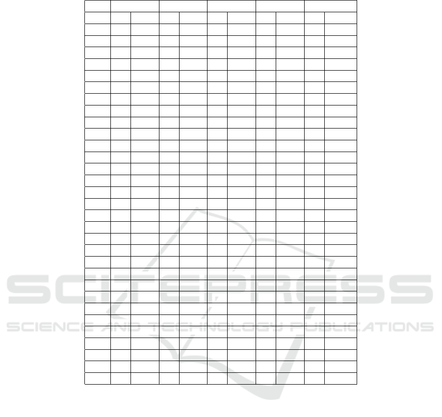
Table 3: Comparison of non dominated solutions sets of Bee-route and evolutionary algorithms on the RC1 instances set.

Bee-route MOV-GP Best Known KBEA Modiﬁed ABC

NV T.dis NV T.dis NV T.dis NV T.dis NV T.dis

RC101 14 1696.9 14 1650.1

15 1636.5 15 1690.6 15 1624.9

16 1629.4 16 1678.9 16 1634.5

17 1615.2

RC102 11 1586.0

12 1571.18 12 1554.7 12 1554.7

13 1509.4 13 1477.5

14 1442.0 14 1461.3

15 1493.2 15 1492.8

RC103 11 1261.6 11 1261.6

12 1331.8

13 1334.5

14 1273.9

RC104 10 1153.5 10 1135.4 10 1135.4

11 1147.7 11 1177.2 11 1215.6

12 1126.7

RC105 13 1629.4 13 1629.4

14 1592.7 14 1540.1

15 1578.5 15 1611.5 15 1519.2 15 1546.4

16 1536.5 16 1589.4 16 1518.6

RC106 11 1424.7 11 1424.7

12 1385.2 12 1394.4

13 1362.9 13 1437.6 13 1377.3

14 1351.1 14 1425.3 14 1423.1

RC107 11 1222.1 11 1230.4 11 1222.1

12 1263.0 12 1212.8 12 1300

13 1229.7

RC108 9 1153.8

10 1141.2 10 1139.8 10 1139.8

11 1111.2 11 1156.5 11 1117.5

12 1193.6

4.4 Statistical Test

We perform in this section a statistical test to verify

if the results returned by Bee-route are signiﬁcantly

better than those returned by the the algorithms MOV-

GP (Ghoseiri and Ghannadpour, 2010), IABC (Yao,

2017), Modiﬁed ABC (Alzaqebah and Sana, 2016)

and KBEA (Tsung-Che and Wei-Huai, 2014). We use

the Wilcoxon test (Riquelme and Baran, 2005) with a

level of signiﬁcance (α = 0.05). We test the set of

non-dominated solutions of all instances of R1, R2,

RC1 and RC2 since the approximate Pareto sets of

each instance is not large enough to test each instance

separately.

Table 6 shows that Bee-route algorithm returns

non dominated solutions that are signiﬁcantly better

than the other evolutionary algorithms almost for

all the instances in both the objectives Number of

Vehicles (N.v) and Total distance (T.d). Thus, the

Wilcoxon Test conﬁrms the performance of our algo-

rithm and show that our algorithm is signiﬁcantly bet-

ter when compared to the state-of-the-art algorithms

for the multi-objective VRPTW except for some in-

stances where the results are very close and the dif-

ference is not signiﬁcant.

4.5 CPU Time Comparison

Table 7 shows the average computation time, the

number of runs, and the computing environment for

the compared algorithms Bee-route, MOV-GP (Gho-

seiri and Ghannadpour, 2010), IABC (Yao, 2017) and

KBEA (Tsung-Che and Wei-Huai, 2014). We note

that these values are given as an indication since the

Bee-route: A Bee Algorithm for the Multi-objective Vehicle Routing Problem

315

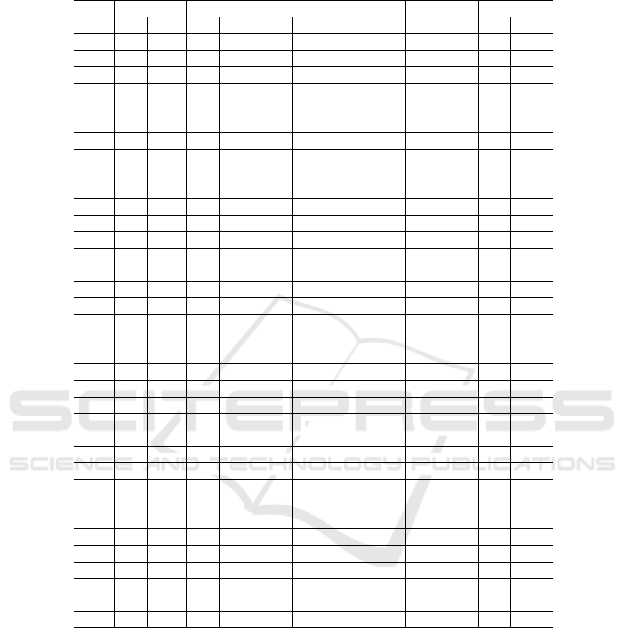
Table 4: Comparison of non dominated solutions sets of Bee-route and evolutionary algorithms on the RC2 instances set.

Bee-route MOV-GP Best Known KBEA IABC Modiﬁed ABC

NV T.dis NV T.dis NV T.dis NV T.dis NV T.dis NV T.dis

RC201 4 1423.7 4 1406.9 4 1406.9 4 1258.6

5 1298.9 5 1279.6

6 1279.9

7 1254.3 7 1273.5

8 1272.2 8 1308.7

RC202 3 1384.1 3 1365.6 3 1365.6

4 1057.7 4 1369.8 4 1162.5

5 1118.6

6 1020.1

8 1099.5 8 1167

RC203 3 1069.1 3 1049.6 3 1049.6 3 1083.6

4 1045.4 4 1060 4 945.1

5 1039.1 5 926.8

6 906.5 6 1014.7

RC204 2 926.5

3 819.3 3 901.4 3 798.4 3 798.4 3 799.1

4 788.6 4 881.8

RC205 4 1282.2 4 1410.3 4 1297.6 4 1297.6 4 1321.3

5 1246.2 5 1236.7

6 1187.9

7 1161.8 7 1210.6

RC206 3 1146.3 3 1146.3 3 1171.2

4 1095.7 4 1194.8 4 1081.8

5 1012.6 5 1068.7

6 1112.3

7 1054.6

RC207 2 1028.9

3 1014.5 3 1061.1 3 1061.1 3 1096.5

4 998.7 4 1040.6 4 1001.8

5 982.5

6 966.3

7 1059.6

RC208 2 909.1

3 856.4 3 898.5 3 828.1 3 828.1 3 833.9

4 845.9 4 783.1

5 882.1

different algorithms are tested on different comput-

ers. However, Bee-route demonstrates the ability to

produce high quality solutions in shorter CPU times.

5 CONCLUSION

This article proposes a Bee-route algorithm based on

the artiﬁcial bee colony metaheuristic for the multi-

objective vehicle routing problem with time win-

dow. The proposed algorithm Bee-route is applied

on a well-known benchmark of VRPTW. Experiments

show that the algorithm returns non dominated solu-

tions that are signiﬁcantly better than those obtained

by evolutionary algorithms from the state of the art

and also the best solution reported by the benchmarks.

In fact the non-dominated solutions returned by Bee-

route dominate those returned by the other algorithms

for most of the tested instances.

The proposed algorithm ﬁnds the largest approximate

Pareto sets almost at all times, and a well distributed

front. But KBEA ﬁnds a set of non-dominated

solutions larger than that of D-MABC for 18 in-

stances. However, hybridizing our algorithm with

ICSOFT 2020 - 15th International Conference on Software Technologies

316

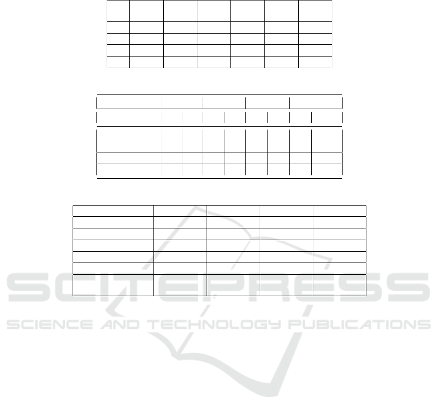
Table 5: Hypervolume metric values for Bee-route and evolutionary algorithms.

Bee-

route

MOV-

Best-

Known

KBEA IABC Modiﬁed

ABC

R1 6.71E+05 6.70E+05 5.96E+05 6.60E+05 4.67E+05 6.57E+05

R2 8.31E+04 4.20E+04 2.00E+04 9.54E+04 n/a 7.58E+04

RC1 4.72E+05 4.32E+05 3.33E+05 4.60E+05 n/a 4.18E+05

RC2 8.56E+04 4.32E+04 2.25E+04 8.37E+04 2.11E+04 8.37E+04

Table 6: Comparative set of distance solutions in Bee-route and evolutionary algorithms with Wilcoxon Test.

W.TEST MOV-GP KBEA IABC Modiﬁed ABC

N.v T.d N.v T.d N.v T.d N.v T.d

Bee-route R1 + + + + + + + +

Bee-route R2 + + + - n/a n/a + +

Bee-route RC1 + + + + n/a n/a + +

Bee-route RC2 + + + + + + + +

Table 7: Average computation time, computing environments, and number of runs.

Algorithm MOV-GP KBEA Bee-route IABC

Avg comput time (s.) R1 > 500 11.7 9.9 39.98

R2 > 900 22.7 16.2 n/a

RC1 > 500 10.4 7.6 n/a

RC2 > 1300 19.1 10.3 22.5

runs 10 10 10 20

CPU/Language 1.6

GHz(Matlab)

Intel i7-3770

3.4 GHz (C++)

Intel i5-2520M

2.5 GHz (C++)

n/a

other heuristics could diversify more the approximate

Pareto sets and large the number of non dominated

solutions. Bee-route could also be a promising ap-

proach for other multi-objective problems with more

than two objectives to optimize. In future works, we

want to combine our algorithm with other heuristics

of the state of the art. We can combine the ABC algo-

rithm with other metaheuristics in order to widen the

space of the Pareto front. Also we can solve other ver-

sions of the problem of VRP like the Vehicle Routing

Problem with Pickup and Delivery, the Vehicle Rout-

ing Problem with Multiple Trips, the Open Vehicle

Routing Problem, etc.

REFERENCES

Alaya I., Sammoud O., H. M. G. K. (2003). Ant colony

optimization for the k-graph partitioning problem. In

The 3rd Tunisia-Japan Symposium on Science and

Technology (TJASST).

Alzaqebah, Malek. Salwani, A. and Sana, J. (2016). Modi-

ﬁed artiﬁcial bee colony for the vehicle routing prob-

lems with time windows. In SpringerPlus. 5(1398),

1-12.

Alzaqebah, M., Jawarneh, S., Sarim, H. M., and Abdullah,

S. (2018). Bees algorithm for vehicle routing prob-

lems with time windows. International Journal of Ma-

chine Learning and Computing, 8(3):236–240.

aysy, O. and Gendreau, M. (2005). Vehicle routing prob-

lem with time windows, part i: Route construction and

local search algorithms. In Transportation science.

39(1), 104-118.

Ghaleini E. N., Koopialipoor M., M. M. S. M. E. M. T. G. B.

(2018). A combination of artiﬁcial bee colony and

neural network for approximating the safety factor of

retaining walls. In Engineering with Computers. 8(8),

1-12.

Ghoseiri, K. and Ghannadpour, S. (2010). Multi-objective

vehicle routing problem with time windows using goal

programming and genetic algorithm. In Applied Soft

Computing. 10(4), 1096-1107.

Lim, A. and Zhang, X. (2007). A two-stage heuristic with

ejection pools and generalized ejection chains for the

vehicle routing problem with time windows. In IN-

FORMS Journal on Computing. 19(3), 443-457.

Riquelme, N., V. L. C. and Baran, B. (2005). Perfor-

mance metrics in multi-objective optimization. In

Latin American Comp. Conf. (CLEI). 10(13), 1-11.

Shaoqiang, Y. Cuicui, T. Y. L. and Linjie, G. (2016). An im-

proved artiﬁcial bee colony algorithm for vehicle rout-

ing problem with time windows, a real case in dalian.

In Advances in Mechanical Engineering. 8(8), 1-9.

Solomon, M. (1987). Algorithms for the vehicle routing and

Bee-route: A Bee Algorithm for the Multi-objective Vehicle Routing Problem

317

scheduling problem. In Operations Research. 35(2),

254-265.

Tsung-Che, C. and Wei-Huai, H. (2014). A knowledge-

based evolutionary algorithm for the multiobjective

vehicle routing problem with time windows. In Com-

puters and Operations Research. 45(4), 25-37.

Yao, B. Yan, Q. Z. M. Y. Y. (2017). Improved artiﬁcial

bee colony algorithm for vehicle routing problem with

time windows. In PLoS ONE. 12(9).

Zitzler, E., r. (2001). Hypervolume met-

ric calculation. In Computer Engi-

neering and Networks Laboratory (TIK).

ftp://ftp.tik.ee.ethz.ch/pub/people/zitzler/hypervol.c.

Zouari W., Alaya I., T. M. (2017). A hybrid ant colony al-

gorithm with a local search for the strongly correlated

knapsack problem. In AIEEE/ACS 14th International

Conference on Computer Systems and Applications.

527-533.

ICSOFT 2020 - 15th International Conference on Software Technologies

318